G 16 4427 Practical MRI 1 Introduction to

G 16. 4427 Practical MRI 1 Introduction to the course Mathematical fundamentals G 16. 4427 Practical MRI 1 – 29 th January 2015

Course Summary • Practical introduction to the basic components of signal detection and excitation in magnetic resonance imaging (MRI) • Organized in 3 modules (lectures + labs): – Part 1 Fundamental mathematical tools needed to describe an MRI experiment and their implementation in Matlab – Part 2 Basic concepts of MR pulse sequences – Part 3 Principles of RF coil design and development G 16. 4427 Practical MRI 1 – 29 th January 2015

Course Information • Website: – https: //alex. med. nyu. edu/portal/site/practicalmri 1 • Format – Twice per week from the 29 th January to 7 th May – 15 120 -mins lectures, 10 240 -mins labs, 2 exams – All sessions at the Center for Biomedical Imaging • Grading policy: – Course participation (10%), midterm exam (25%), lab projects (40%), final exam (25%) • Reference textbooks – J. T. Vaughan and J. R. Griffiths RF coils for MRI, Wiley -Liss, 2012 – M. A. Bernstein, K. F. King and X. J. Zhou, Handbook of MRI Pulse Sequences, Academic Press, 2004 G 16. 4427 Practical MRI 1 – 29 th January 2015

Instructors • Prof. Riccardo Lattanzi (course director) – All lectures and first lab session – Riccardo. Lattanzi@nyumc. org (212 -263 -4860) – Office hours: after class or by appointment • Prof. Kaveh Vahedipour – Pulse sequence programming lab sessions – Kaveh. Vahedipour@nyumc. org • Dr. Ryan Brown – RF coil lab sessions – Ryan. Brown@nyumc. org G 16. 4427 Practical MRI 1 – 29 th January 2015

Matlab • NYU has an institutional license • Installation instructions with license info are also posted on the course website on ALEX • If you have one, bring your laptop with Matlab for next class G 16. 4427 Practical MRI 1 – 29 th January 2015

Any questions? G 16. 4427 Practical MRI 1 – 29 th January 2015

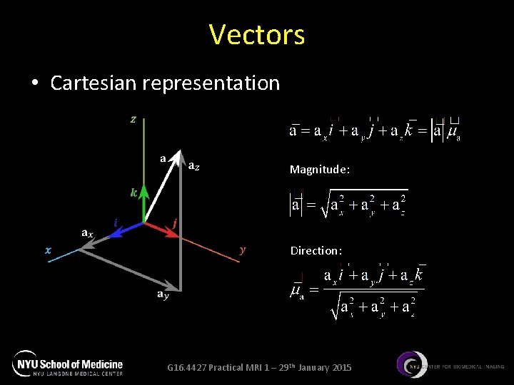
Vectors • Cartesian representation Magnitude: Direction: G 16. 4427 Practical MRI 1 – 29 th January 2015

Question: Can you provide examples of vectors quantity in MRI? G 16. 4427 Practical MRI 1 – 29 th January 2015

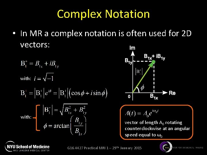
Complex Notation • In MR a complex notation is often used for 2 D vectors: with: vector of length A 0 rotating counterclockwise at an angular speed equal to ω0 G 16. 4427 Practical MRI 1 – 29 th January 2015

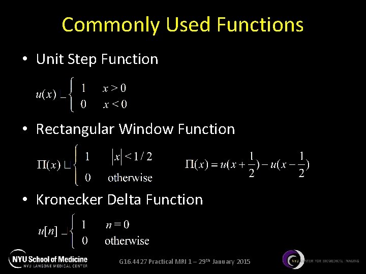
Commonly Used Functions • Unit Step Function • Rectangular Window Function • Kronecker Delta Function G 16. 4427 Practical MRI 1 – 29 th January 2015

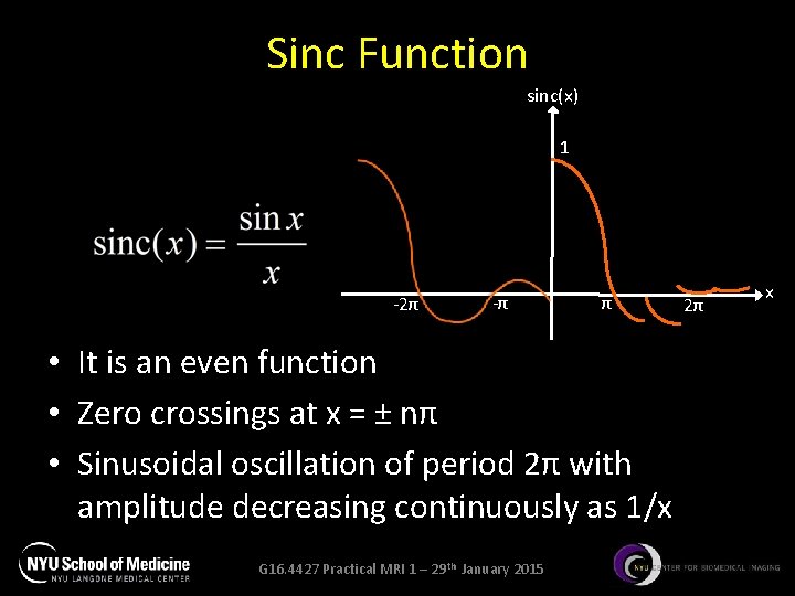
Sinc Function sinc(x) 1 -2π -π π • It is an even function • Zero crossings at x = ± nπ • Sinusoidal oscillation of period 2π with amplitude decreasing continuously as 1/x G 16. 4427 Practical MRI 1 – 29 th January 2015 2π x

Any questions? G 16. 4427 Practical MRI 1 – 29 th January 2015

Matlab Demonstration G 16. 4427 Practical MRI 1 – 29 th January 2015

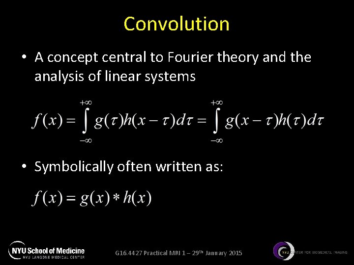
Convolution • A concept central to Fourier theory and the analysis of linear systems • Symbolically often written as: G 16. 4427 Practical MRI 1 – 29 th January 2015

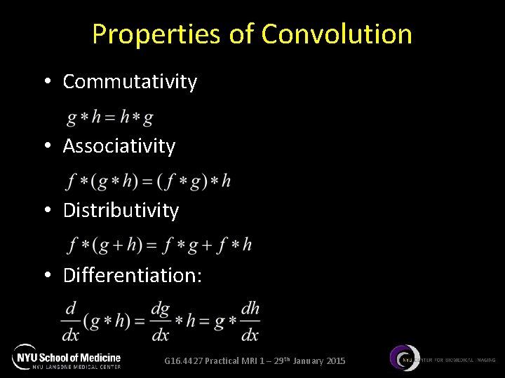
Properties of Convolution • Commutativity • Associativity • Distributivity • Differentiation: G 16. 4427 Practical MRI 1 – 29 th January 2015

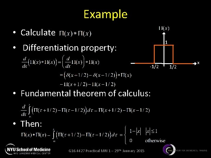
Example • Calculate 1 • Differentiation property: -1/2 • Fundamental theorem of calculus: • Then: G 16. 4427 Practical MRI 1 – 29 th January 2015 1/2 x

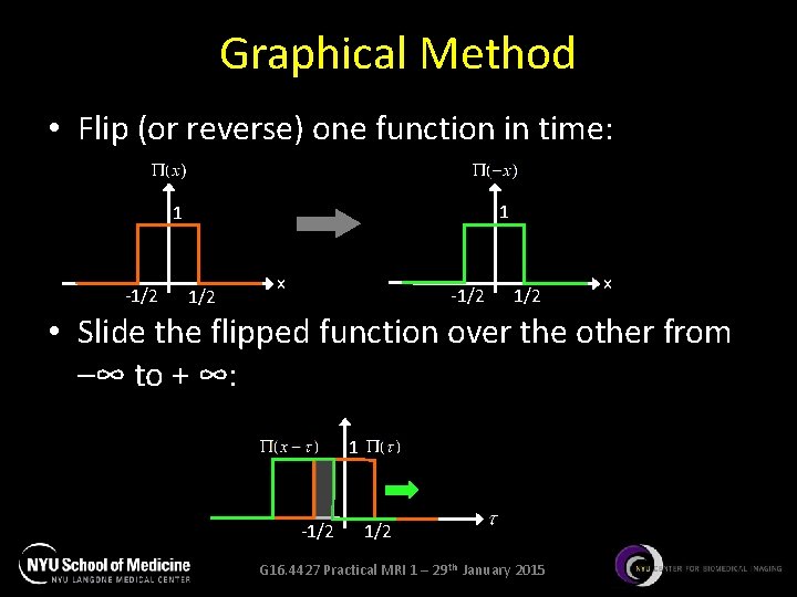
Graphical Method • Flip (or reverse) one function in time: 1 1 -1/2 1/2 x • Slide the flipped function over the other from –∞ to + ∞: 1 -1/2 G 16. 4427 Practical MRI 1 – 29 th January 2015

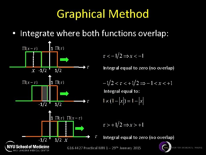
Graphical Method • Integrate where both functions overlap: 1 -1/2 Integral equal to zero (no overlap) 1 Integral equal to: -1/2 1 -1/2 Integral equal to zero (no overlap) G 16. 4427 Practical MRI 1 – 29 th January 2015

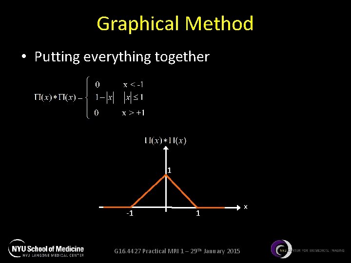
Graphical Method • Putting everything together 1 -1 1 G 16. 4427 Practical MRI 1 – 29 th January 2015 x

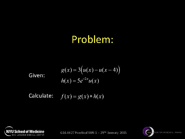
Problem: Given: Calculate: G 16. 4427 Practical MRI 1 – 29 th January 2015

Matlab Demonstration G 16. 4427 Practical MRI 1 – 29 th January 2015

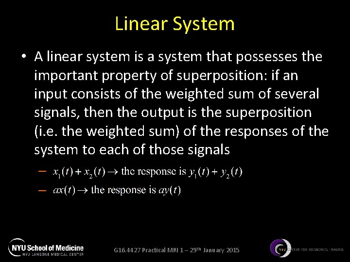
Linear System • A linear system is a system that possesses the important property of superposition: if an input consists of the weighted sum of several signals, then the output is the superposition (i. e. the weighted sum) of the responses of the system to each of those signals – – G 16. 4427 Practical MRI 1 – 29 th January 2015

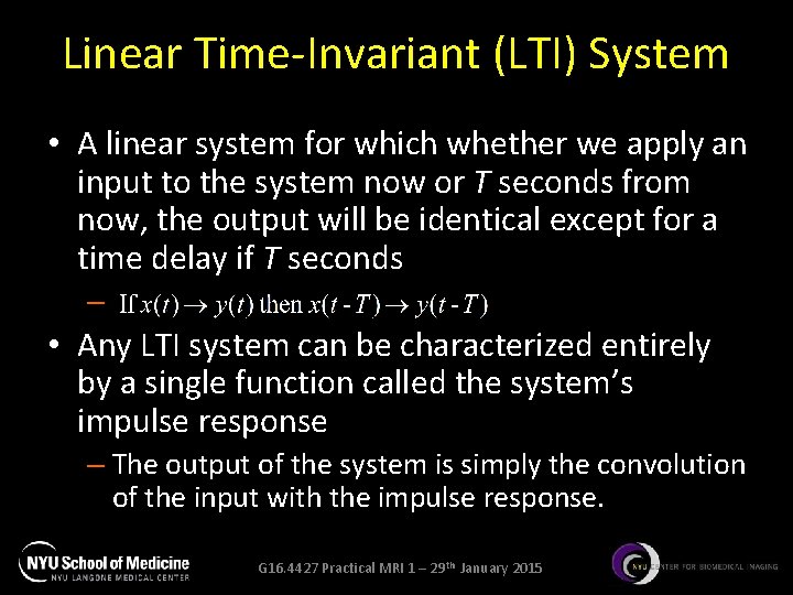
Linear Time-Invariant (LTI) System • A linear system for which whether we apply an input to the system now or T seconds from now, the output will be identical except for a time delay if T seconds – • Any LTI system can be characterized entirely by a single function called the system’s impulse response – The output of the system is simply the convolution of the input with the impulse response. G 16. 4427 Practical MRI 1 – 29 th January 2015

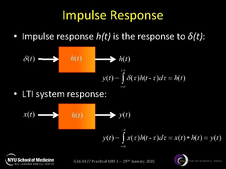
Impulse Response • Impulse response h(t) is the response to δ(t): • LTI system response: G 16. 4427 Practical MRI 1 – 29 th January 2015

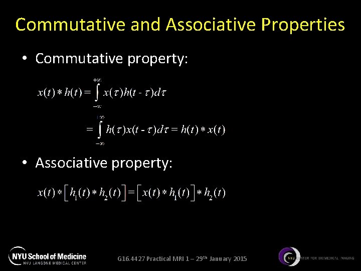
Commutative and Associative Properties • Commutative property: • Associative property: G 16. 4427 Practical MRI 1 – 29 th January 2015

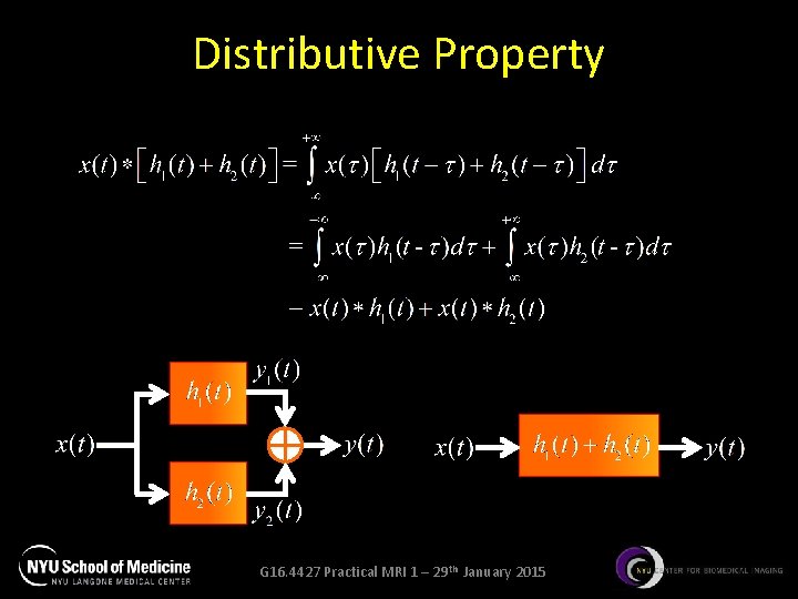
Distributive Property G 16. 4427 Practical MRI 1 – 29 th January 2015

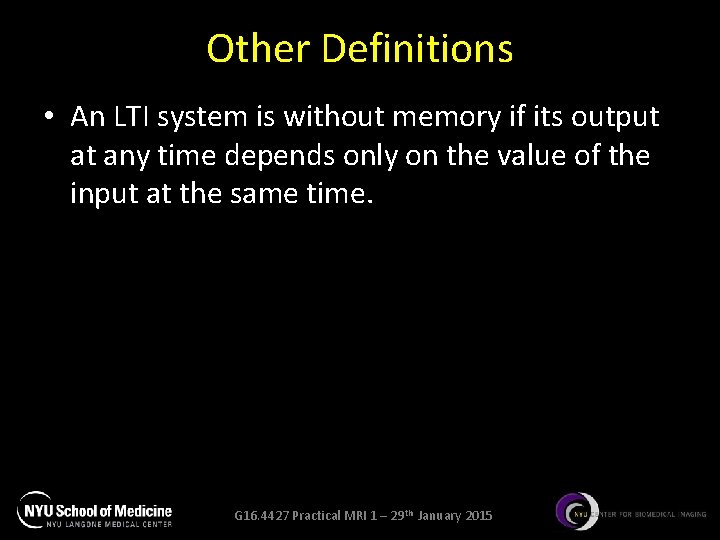
Other Definitions • An LTI system is without memory if its output at any time depends only on the value of the input at the same time. G 16. 4427 Practical MRI 1 – 29 th January 2015

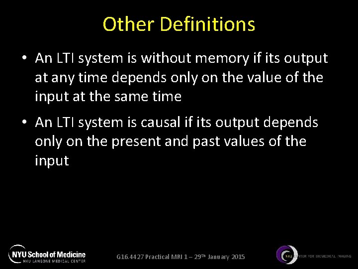
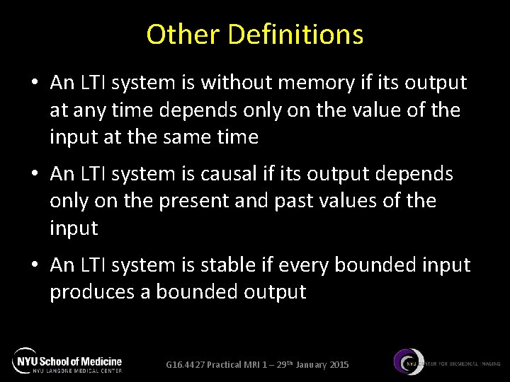
Other Definitions • An LTI system is without memory if its output at any time depends only on the value of the input at the same time • An LTI system is causal if its output depends only on the present and past values of the input G 16. 4427 Practical MRI 1 – 29 th January 2015

Other Definitions • An LTI system is without memory if its output at any time depends only on the value of the input at the same time • An LTI system is causal if its output depends only on the present and past values of the input • An LTI system is stable if every bounded input produces a bounded output G 16. 4427 Practical MRI 1 – 29 th January 2015

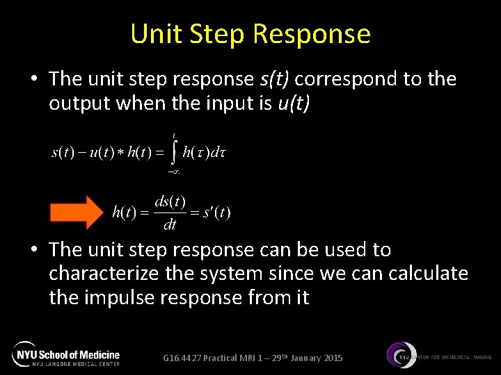
Unit Step Response • The unit step response s(t) correspond to the output when the input is u(t) • The unit step response can be used to characterize the system since we can calculate the impulse response from it G 16. 4427 Practical MRI 1 – 29 th January 2015

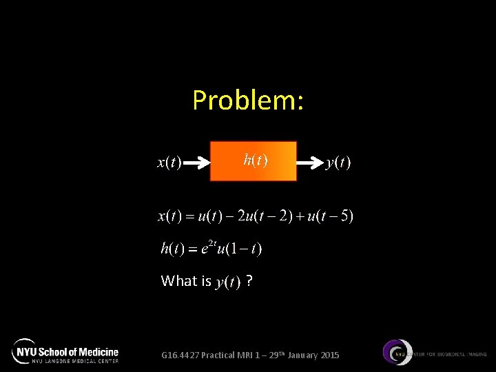
Problem: What is ? G 16. 4427 Practical MRI 1 – 29 th January 2015

Any questions? G 16. 4427 Practical MRI 1 – 29 th January 2015

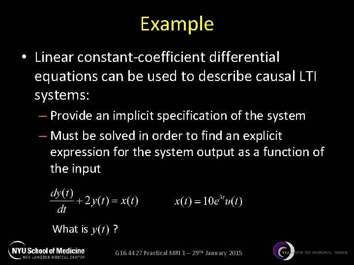
Example • Linear constant-coefficient differential equations can be used to describe causal LTI systems: – Provide an implicit specification of the system – Must be solved in order to find an explicit expression for the system output as a function of the input What is ? G 16. 4427 Practical MRI 1 – 29 th January 2015

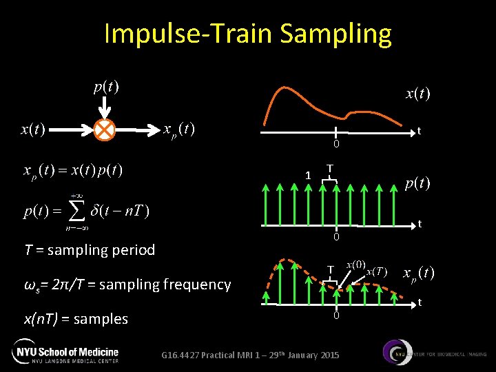
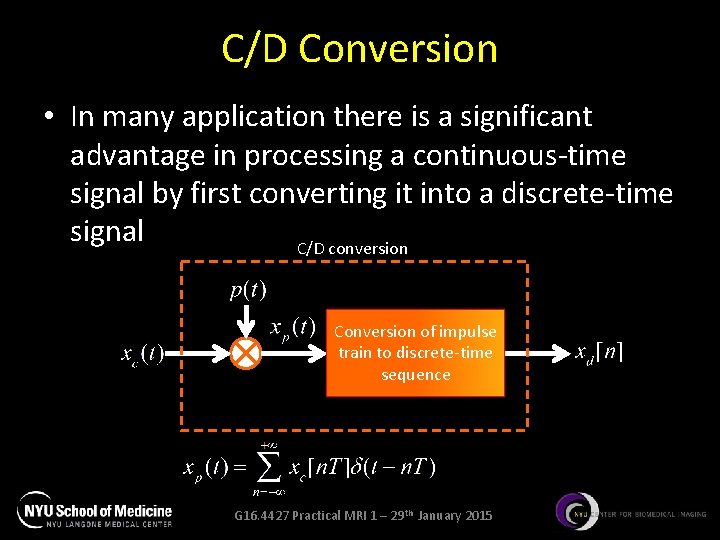
Sampling • Under certain conditions, a continuous-time signal can be completely represented by and recoverable from knowledge of its samples at points equally spaced in times • A convenient way to sample a continuoustime signal x(t) is to multiply it by a periodic impulse train p(t) (i. e. the sampling function) • In MRI sampling is very important! G 16. 4427 Practical MRI 1 – 29 th January 2015

Question: Can you provide examples of sampling in MRI? G 16. 4427 Practical MRI 1 – 29 th January 2015

Impulse-Train Sampling 0 1 T 0 T = sampling period ωs= 2π/T = sampling frequency x(n. T) = samples t t T 0 G 16. 4427 Practical MRI 1 – 29 th January 2015 t

C/D Conversion • In many application there is a significant advantage in processing a continuous-time signal by first converting it into a discrete-time signal C/D conversion Conversion of impulse train to discrete-time sequence G 16. 4427 Practical MRI 1 – 29 th January 2015

Discrete-Time Convolution • The input x[n] and the output y[n] of a discrete-time LTI system are related by the convolution sum: • The same properties of the continuous case apply to the discrete case G 16. 4427 Practical MRI 1 – 29 th January 2015

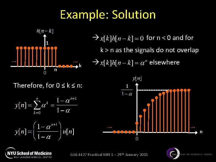
Example: Question • Find y[n] given: with 0 < α < 1 1 … n … 0 G 16. 4427 Practical MRI 1 – 29 th January 2015 n

Example: Solution 1 k > n as the signals do not overlap … … 0 for n < 0 and for n k elsewhere Therefore, for 0 ≤ k ≤ n: … … 0 G 16. 4427 Practical MRI 1 – 29 th January 2015 n

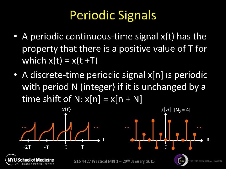
Periodic Signals • A periodic continuous-time signal x(t) has the property that there is a positive value of T for which x(t) = x(t +T) • A discrete-time periodic signal x[n] is periodic with period N (integer) if it is unchanged by a time shift of N: x[n] = x[n + N] (N 0 = 4) … … n t -2 T -T 0 T G 16. 4427 Practical MRI 1 – 29 th January 2015 0

Matlab Demonstration G 16. 4427 Practical MRI 1 – 29 th January 2015

See you on Tuesday! G 16. 4427 Practical MRI 1 – 29 th January 2015