FW 364 Ecological Problem Solving Class 5 Population
FW 364 Ecological Problem Solving Class 5: Population Growth Sept. 16, 2013
Outline for Today Goal for Today: Introduction to population growth – Discrete Growth Objective for Today: Derive a simple model of discrete population growth between consecutive time periods (Nt and Nt+1) Objective for Next Class: Derive an equation to forecast population growth (still discrete growth) Objective for Class after Next: Derive continuous population growth equation Text (optional reading): Next three classes correspond to Chapter 1
Muskox Case Study 1700 -1800 s: Excessive hunting eliminated muskox from most of their natural North American range 1850 -1860: Last individuals killed in Alaska Ovibos moschatus 1930: Territory of Alaska Legislature authorized re-introduction from Greenland 31 muskox to 1936: Nunivak Island introduced to Nunivak Island 1965: Population size of 514 muskox! 1965 -1968: 48 animals removed for reintroductions elsewhere in Alaska Nunivak Island Great opportunity for population analysis because:
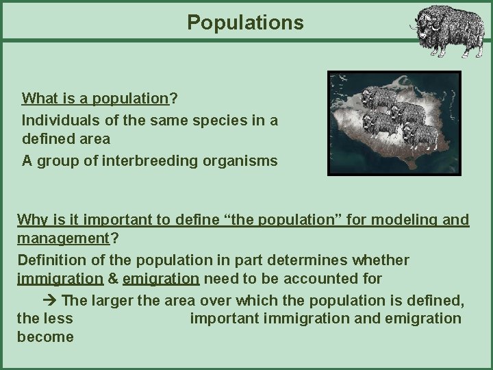
Populations What is a population? Individuals of the same species in a defined area A group of interbreeding organisms Why is it important to define “the population” for modeling and management? Definition of the population in part determines whether immigration & emigration need to be accounted for The larger the area over which the population is defined, the less important immigration and emigration become
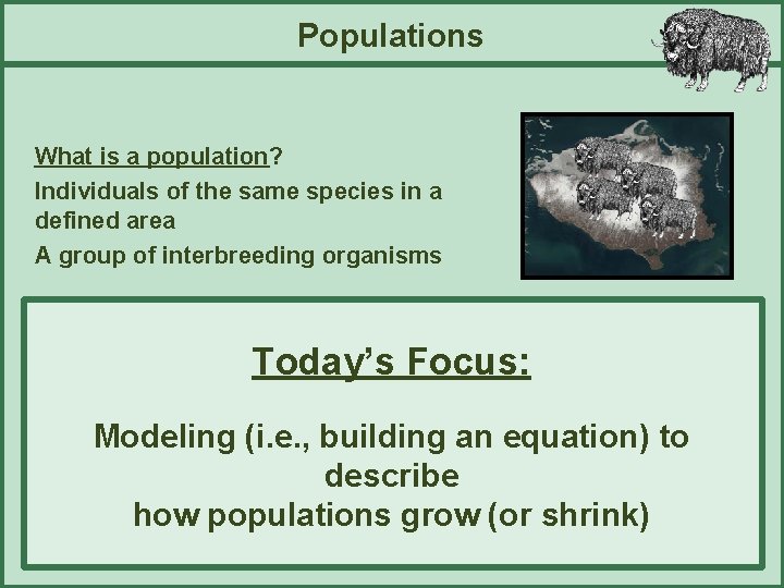
Populations What is a population? Individuals of the same species in a defined area A group of interbreeding organisms Why is it important to define “the population” for modeling and Today’s Focus: management? Definition of the population in part determines whether Modeling (i. e. , building an equation) to immigration & emigration need to be accounted for The larger the area over which the population is defined, describe the less how populations importantgrow immigration and emigration (or shrink) become

Basic Population Growth General form: Density at time in future = function of density at present time Nt+1 = f(Nt) Nt = density of the population at time t (e. g. , year 3 or day 12) Nt+1 = density of the population at time t+1 (e. g. , year 3+1 or day 12+1) f(Nt) means a function “dependent on Nt” Note: It is common to refer to Nt and Nt+1 as “densities” because we are working with abundance in a pre-determined area [remember the definition of a population] However, the spatial aspect is implicit in the model … We’ll treat Nt and Nt+1 as abundances (i. e. , numbers of individuals)
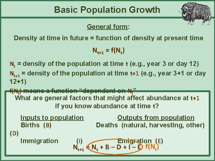
Basic Population Growth General form: Density at time in future = function of density at present time Nt+1 = f(Nt) Nt = density of the population at time t (e. g. , year 3 or day 12) Nt+1 = density of the population at time t+1 (e. g. , year 3+1 or day 12+1) f(Nt) means a function “dependent on Nt” What are general factors that might affect abundance at t+1 if you know abundance at time t? Inputs to population Births (B) Outputs from population Deaths (natural, harvesting, other) (D) Immigration (I) Emigration (E) Nt+1 = Nt + B – D + I – E f(Nt)
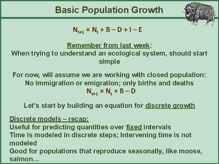
Basic Population Growth Nt+1 = Nt + B – D + I – E Remember from last week: When trying to understand an ecological system, should start simple For now, will assume we are working with closed population: No immigration or emigration; only births and deaths Nt+1 = Nt + B – D Let’s start by building an equation for discrete growth Discrete models – recap: Useful for predicting quantities over fixed intervals Time is modeled in discrete steps; Intervening time is not modeled Good for populations that reproduce seasonally, like moose, salmon…

Basic Population Growth 1965 -1968: Removals 1936: First introduction Population closed to immigration / emigration So we can use Nt+1 = Nt + B – D to model muskox population size at discrete intervals Fig 1. 3 in text e. g. , one year to the next Plot curves upward: Suggestive of “multiplicative growth”, but not diagnostic (we’ll check later) Multiplicative (geometric) growth: population size increases (or decreases) by a constant fraction per year (rather than adding,
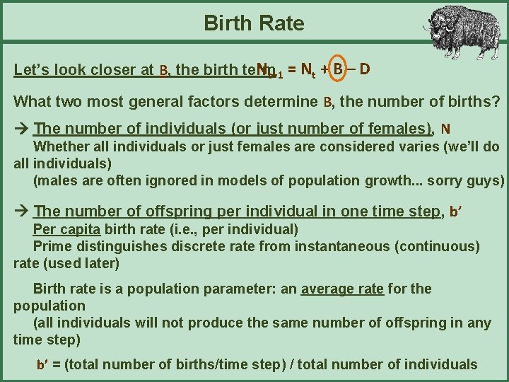
Birth Rate Nt+1 = Nt + B – D Let’s look closer at B, the birth term What two most general factors determine B, the number of births? The number of individuals (or just number of females), N Whether all individuals or just females are considered varies (we’ll do all individuals) (males are often ignored in models of population growth. . . sorry guys) The number of offspring per individual in one time step, b’ Per capita birth rate (i. e. , per individual) Prime distinguishes discrete rate from instantaneous (continuous) rate (used later) Birth rate is a population parameter: an average rate for the population (all individuals will not produce the same number of offspring in any time step) b’ = (total number of births/time step) / total number of individuals
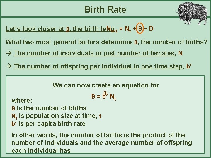
Birth Rate Nt+1 = Nt + B – D Let’s look closer at B, the birth term What two most general factors determine B, the number of births? The number of individuals or just number of females, N The number of offspring per individual in one time step, b’ We can now create an equation for B: B = b’ Nt where: B is the number of births Nt is population size at time, t b’ is per capita birth rate In other words, the number of births is the product of the number of individuals and the average number of offspring each individual has
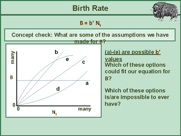
Birth Rate B = b’ Nt Concept check: What are some of the assumptions we have made for B? many b e B d 0 0 Nt c a many (a)-(e) are possible b’ values Which of these options could fit our equation for B? Which of these options is/are impossible to ever have?
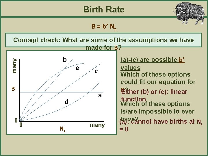
Birth Rate B = b’ Nt Concept check: What are some of the assumptions we have made for B? many b e B d 0 0 Nt c a many (a)-(e) are possible b’ values Which of these options could fit our equation for B ? Either (b) or (c): linear function Which of these options is/are impossible to ever have? (a): cannot have births at N =0 t
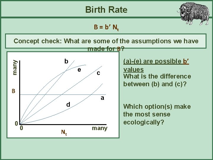
Birth Rate B = b’ Nt Concept check: What are some of the assumptions we have made for B? many e B d 0 (a)-(e) are possible b’ values What is the difference between (b) and (c)? b 0 Nt c a many Which option(s) make the most sense ecologically?
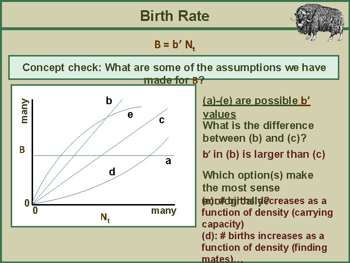
Birth Rate B = b’ Nt Concept check: What are some of the assumptions we have made for B? many b e B d 0 0 Nt c a many (a)-(e) are possible b’ values What is the difference between (b) and (c)? b’ in (b) is larger than (c) Which option(s) make the most sense (e): # births decreases as a ecologically? function of density (carrying capacity) (d): # births increases as a function of density (finding mates)…
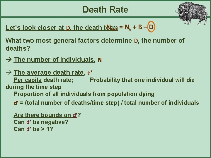
Death Rate Nt+1 = Nt + B – D Let’s look closer at D, the death term What two most general factors determine D, the number of deaths? The number of individuals, N à The average death rate, d’ Per capita death rate; Probability that one individual will die during the time step Proportion of all individuals from population dying d’ = (total number of deaths/time step) / total number of individuals Are there bounds on d’? Can d’ be negative? Can d’ be > 1?
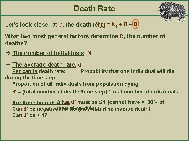
Death Rate Nt+1 = Nt + B – D Let’s look closer at D, the death term What two most general factors determine D, the number of deaths? The number of individuals, N à The average death rate, d’ Per capita death rate; Probability that one individual will die during the time step Proportion of all individuals from population dying d’ = (total number of deaths/time step) / total number of individuals Are there bounds on. No, d’? d’ must be ≤ 1 (cannot have >100% of population dying) Can d’ be negative? No (that would be inverse death) Can d’ be > 1?
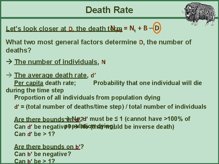
Death Rate Nt+1 = Nt + B – D Let’s look closer at D, the death term What two most general factors determine D, the number of deaths? The number of individuals, N à The average death rate, d’ Per capita death rate; Probability that one individual will die during the time step Proportion of all individuals from population dying d’ = (total number of deaths/time step) / total number of individuals Are there bounds on. No, d’? d’ must be ≤ 1 (cannot have >100% of population dying) Can d’ be negative? No (that would be inverse death) Can d’ be > 1? Are there bounds on b’? Can b’ be negative? Can b’ be > 1?
Death Rate Nt+1 = Nt + B – D Let’s look closer at D, the death term What two most general factors determine D, the number of deaths? The number of individuals, N à The average death rate, d’ Per capita death rate; Probability that one individual will die during the time step Proportion of all individuals from population dying d’ = (total number of deaths/time step) / total number of individuals Are there bounds on. No, d’? d’ must be ≤ 1 (cannot have >100% of population dying) Can d’ be negative? No (that would be inverse death) Can d’ be > 1? Individuals can have > 1 Are there bounds on. Absolutely! b’? offspring Can b’ be negative? No (cannot have negative births) Can b’ be > 1?
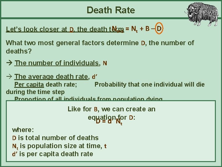
Death Rate Nt+1 = Nt + B – D Let’s look closer at D, the death term What two most general factors determine D, the number of deaths? The number of individuals, N à The average death rate, d’ Per capita death rate; Probability that one individual will die during the time step Proportion of all individuals from population dying d’ = (total number Like of deaths/time / total number of individuals for B, we step) can create an equation for D: D = d’ Nt where: D is total number of deaths Nt is population size at time, t d’ is per capita death rate
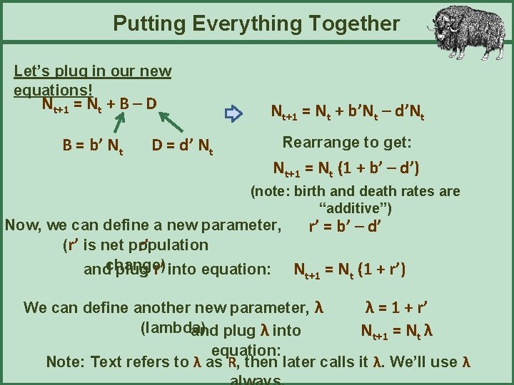
Putting Everything Together Let’s plug in our new equations! Nt+1 = Nt + B – D B = b’ Nt D = d’ Nt Nt+1 = Nt + b’Nt – d’Nt Rearrange to get: Nt+1 = Nt (1 + b’ – d’) (note: birth and death rates are “additive”) Now, we can define a new parameter, r’ = b’ – d’ (r’ is net population r’ andchange) plug r’ into equation: Nt+1 = Nt (1 + r’) We can define another new parameter, λ λ = 1 + r’ (lambda) and plug λ into Nt+1 = Nt λ equation: Note: Text refers to λ as R, then later calls it λ. We’ll use λ
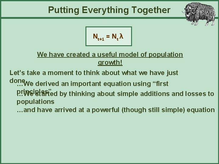
Putting Everything Together Nt+1 = Nt λ We have created a useful model of population growth! Let’s take a moment to think about what we have just done… …We derived an important equation using “first principles” …We started by thinking about simple additions and losses to populations …and have arrived at a powerful (though still simple) equation
Population Growth Break! • Let’s think about birth and death rates in an example population…humans! • http: //www. prb. org/pdf 12/2012 population-data-sheet_eng. pdf
Pick a Country Card • Each card has a country with its birth and death rate. • Using the birth and death rate, calculate net population change and be ready to comment and share: • r’ = b’ – d’
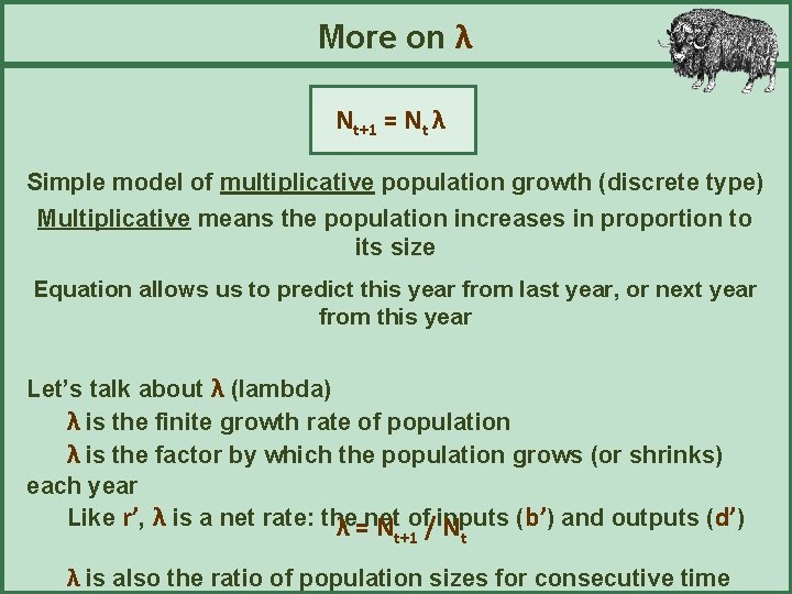
More on λ Nt+1 = Nt λ Simple model of multiplicative population growth (discrete type) Multiplicative means the population increases in proportion to its size Equation allows us to predict this year from last year, or next year from this year Let’s talk about λ (lambda) λ is the finite growth rate of population λ is the factor by which the population grows (or shrinks) each year Like r’, λ is a net rate: the (b’) and outputs (d’) λ =net N of/inputs N t+1 t λ is also the ratio of population sizes for consecutive time
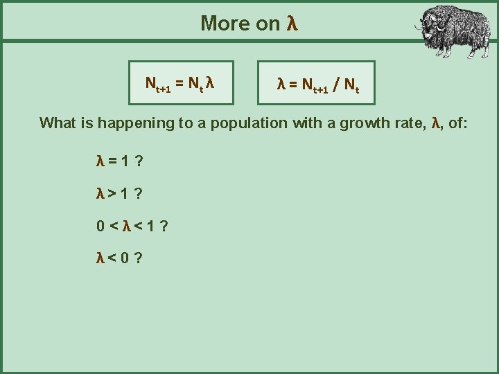
More on λ Nt+1 = Nt λ λ = Nt+1 / Nt What is happening to a population with a growth rate, λ, of: λ=1? λ> 1 ? 0<λ<1? λ< 0 ?
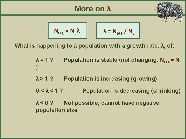
More on λ Nt+1 = Nt λ λ = Nt+1 / Nt What is happening to a population with a growth rate, λ, of: λ=1? ) λ> 1 ? 0 < λ< 1 ? λ< 0 ? Population is stable (not changing, Nt+1 = Nt Population is increasing (growing) Population is decreasing (shrinking) Not possible; cannot have negative population size
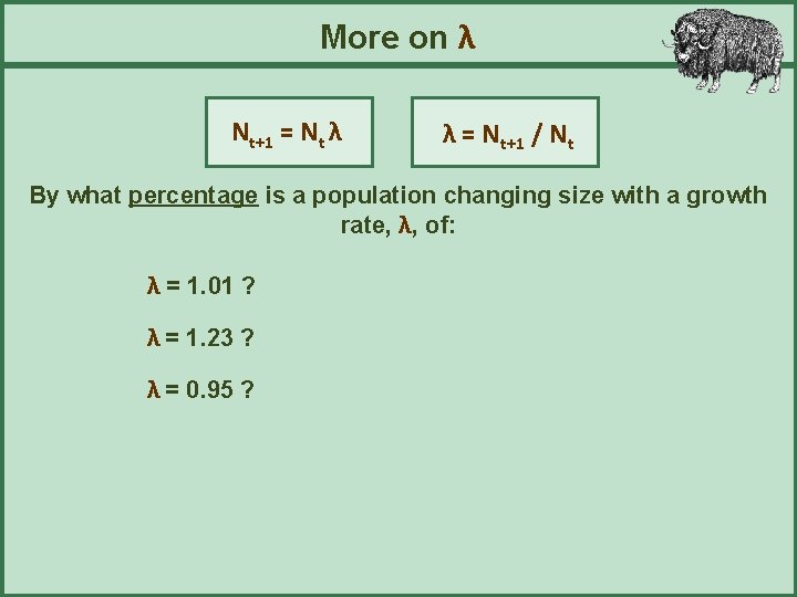
More on λ Nt+1 = Nt λ λ = Nt+1 / Nt By what percentage is a population changing size with a growth rate, λ, of: λ = 1. 01 ? λ = 1. 23 ? λ = 0. 95 ?
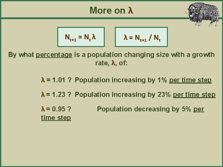
More on λ Nt+1 = Nt λ λ = Nt+1 / Nt By what percentage is a population changing size with a growth rate, λ, of: λ = 1. 01 ? Population increasing by 1% per time step λ = 1. 23 ? Population increasing by 23% per time step λ = 0. 95 ? time step Population decreasing by 5% per
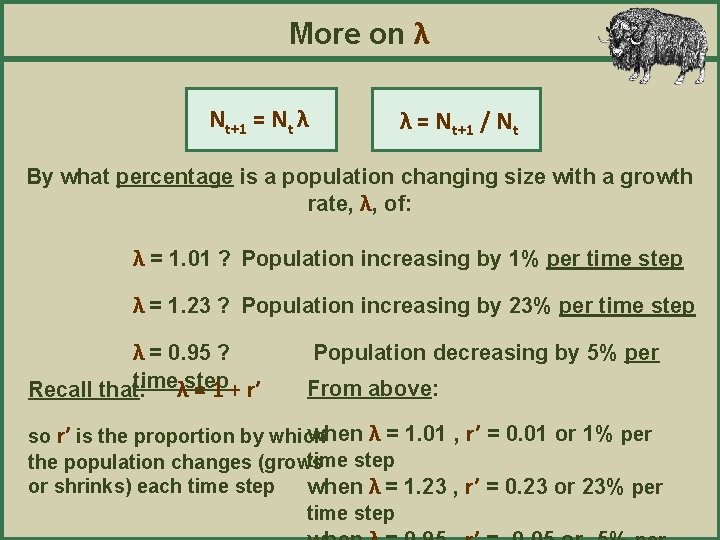
More on λ Nt+1 = Nt λ λ = Nt+1 / Nt By what percentage is a population changing size with a growth rate, λ, of: λ = 1. 01 ? Population increasing by 1% per time step λ = 1. 23 ? Population increasing by 23% per time step λ = 0. 95 ? timeλstep Recall that: = 1 + r’ Population decreasing by 5% per From above: when λ = 1. 01 , r’ = 0. 01 or 1% per so r’ is the proportion by which time step the population changes (grows or shrinks) each time step when λ = 1. 23 , r’ = 0. 23 or 23% per time step
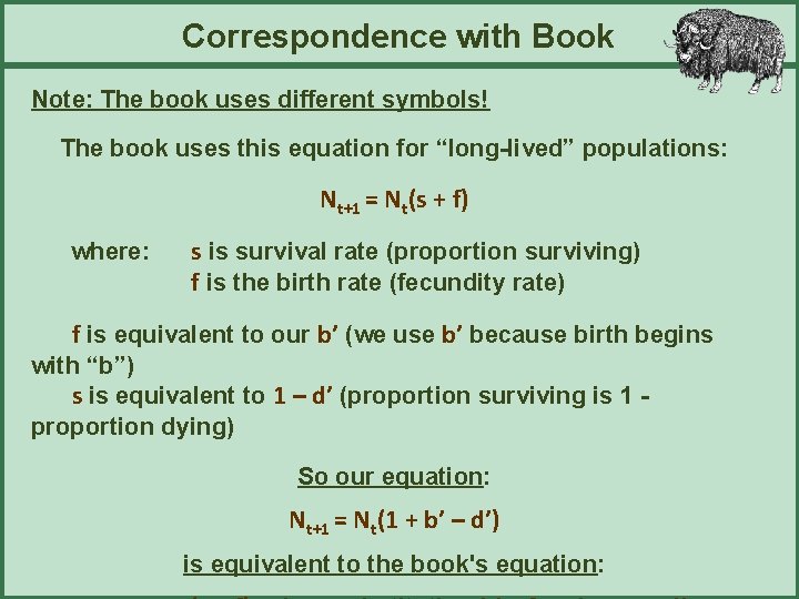
Correspondence with Book Note: The book uses different symbols! The book uses this equation for “long-lived” populations: Nt+1 = Nt(s + f) where: s is survival rate (proportion surviving) f is the birth rate (fecundity rate) f is equivalent to our b’ (we use b’ because birth begins with “b”) s is equivalent to 1 – d’ (proportion surviving is 1 proportion dying) So our equation: Nt+1 = Nt(1 + b’ – d’) is equivalent to the book's equation:
Looking Ahead Next Class: Derive an equation to forecast population growth (still discrete growth) so we can predict population growth between non-consecutive time steps (e. g. , 10 years in the future, not just last year to this year, or this year to next year) Tomorrow: Lab 3 Bring exercise, pencil, paper, and calculator
- Slides: 32