FW 364 Ecological Problem Solving Class 23 Competition

FW 364 Ecological Problem Solving Class 23: Competition November 25, 2013

Outline for Today Shifting focus from predator-prey interactions to two species competition Objectives for Today: Derive equations for two-species resource competition Introduce R* rule to determine competition winner Objectives for Next Three Classes: Explore R* rule in more detail Include Type II functional response for consumers Examine graphical approaches for determining competition winner Discuss limits to competitive exclusion Discuss practical application of resource competition models No textbook chapters!

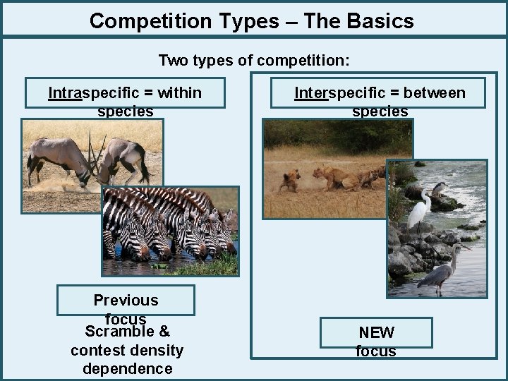
Competition Types – The Basics Two types of competition: Intraspecific = within species Interspecific = between species Previous focus Scramble & contest density dependence NEW focus

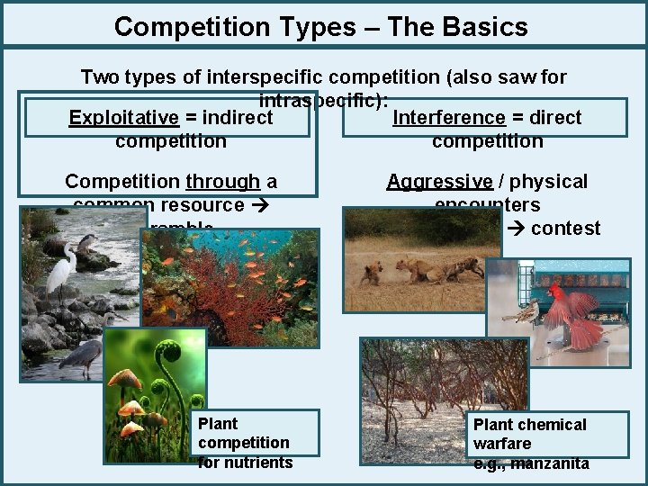
Competition Types – The Basics Two types of interspecific competition (also saw for intraspecific): Interference = direct Exploitative = indirect competition Competition through a common resource scramble Plant competition for nutrients Aggressive / physical encounters for resources contest Plant chemical warfare e. g. , manzanita

Exploitative Interspecific Competition We will only model exploitative interspecific competition a. k. a. resource competition Conceptual framework Consumer 1 Consumer 2 Resource Applies to: Examples: Carnivores-animal prey Herons and cranes competing for fish in swamps Herbivores-plant Zebras and wildebeest consuming grasses Parasites-host Sea lamprey and copepods parasitizing

Exploitative Interspecific Competition C 1 C 2 Key features: R Competition is an extension of predator-prey concepts we just studied! Two coupled predator-prey interactions that share same prey (resource) Interaction between consumers mediated through resource à No direct interaction (this is an assumption!) Only one consumer can persist at steady state (another assumption) à Competitive exclusion principle

Exploitative Interspecific Competition C 1 C 2 Key features: R To reiterate: With the competitive exclusion principle, we are assuming there is always a winner in the long run i. e. , one consumer will out-compete (exclude) the other The winner of the competition is the consumer that is still alive at steady state, whereas the loser is the consumer that has gone extinct

Exploitative Interspecific Competition C 1 C 2 Goals R 1. Determine the competition winner at steady state (algebra) 2. Describe dynamics and forecast time to extinction of inferior competitor (Stella – Lab 10) Important to understand the difference between the two approaches and how they complement each other Let’s build equations! #1 tells us WHO will win #2 tells us WHEN the loser goes extinct, and HOW populations change through time

Competition Equations Like before, we’ll build simple models that capture the essence of two-species resource competition (we’ll be making many assumptions) Start with our basic (coupled) predator-prey equations: Victim, V: d. V/dt = bv. V - dv. V - a. VP Predator, d. P/dt = ac. VP - dp. P P: Adapt more general notation of consumer-resource à substitute R for V, but keep P Note that I will use “consumer” and “predator” interchangeably Resource, d. R/dt = br. R - dr. R - a. RP R: Predator, d. P/dt = ac. RP - dp. P P:

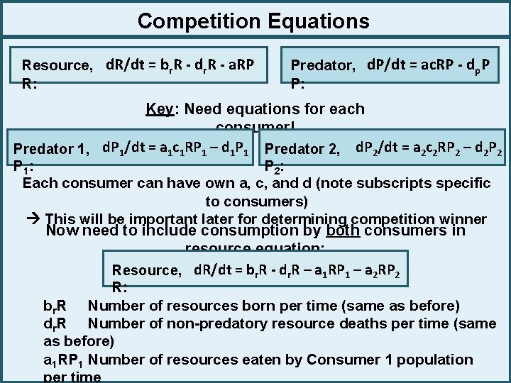
Competition Equations Resource, d. R/dt = br. R - dr. R - a. RP R: Predator, d. P/dt = ac. RP - dp. P P: Key: Need equations for each consumer! Predator 1, d. P 1/dt = a 1 c 1 RP 1 – d 1 P 1 Predator 2, d. P 2/dt = a 2 c 2 RP 2 – d 2 P 2 P 1: P 2: Each consumer can have own a, c, and d (note subscripts specific to consumers) This will be important later for determining competition winner Now need to include consumption by both consumers in resource equation: Resource, d. R/dt = br. R - dr. R – a 1 RP 1 – a 2 RP 2 R: br. R Number of resources born per time (same as before) dr. R Number of non-predatory resource deaths per time (same as before) a 1 RP 1 Number of resources eaten by Consumer 1 population per time

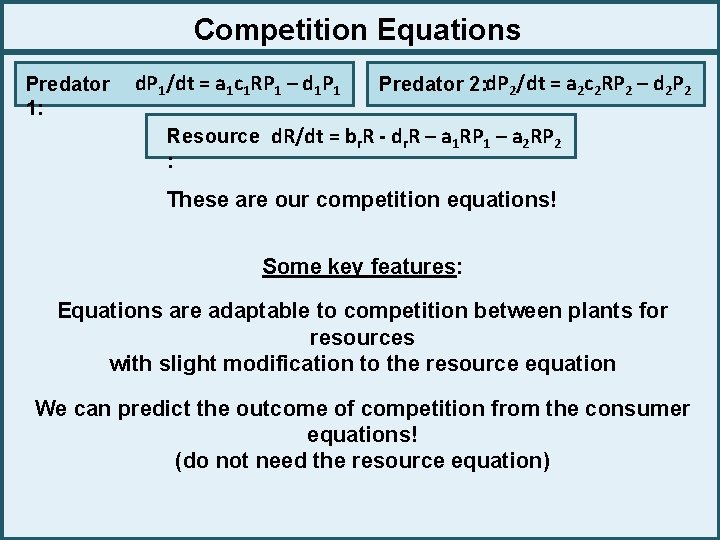
Competition Equations Predator 1: d. P 1/dt = a 1 c 1 RP 1 – d 1 P 1 Predator 2: d. P 2/dt = a 2 c 2 RP 2 – d 2 P 2 Resource d. R/dt = br. R - dr. R – a 1 RP 1 – a 2 RP 2 : These are our competition equations! Some key features: Equations are adaptable to competition between plants for resources with slight modification to the resource equation We can predict the outcome of competition from the consumer equations! (do not need the resource equation)

Competition Equations Predator 1: d. P 1/dt = a 1 c 1 RP 1 – d 1 P 1 Predator 2: d. P 2/dt = a 2 c 2 RP 2 – d 2 P 2 Resource d. R/dt = br. R - dr. R – a 1 RP 1 – a 2 RP 2 : Assumptions: 1. The consumer populations cannot exist if there are no resources 2. In the absence of both consumers, the resources grow exponentially 3. Consumers encounter prey randomly (“well-mixed” environment) 4. Consumers are insatiable (Type I functional response) 5. No age / stage structure 6. Consumers do not interact with each other except through consumption

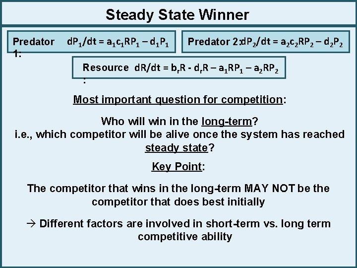
Steady State Winner Predator 1: d. P 1/dt = a 1 c 1 RP 1 – d 1 P 1 Predator 2: d. P 2/dt = a 2 c 2 RP 2 – d 2 P 2 Resource d. R/dt = br. R - dr. R – a 1 RP 1 – a 2 RP 2 : Most important question for competition: Who will win in the long-term? i. e. , which competitor will be alive once the system has reached steady state? Key Point: The competitor that wins in the long-term MAY NOT be the competitor that does best initially à Different factors are involved in short-term vs. long term competitive ability

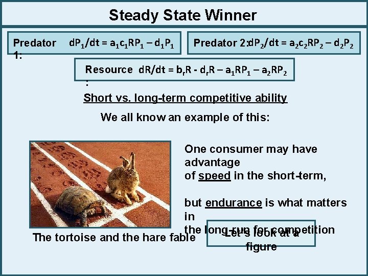
Steady State Winner Predator 1: d. P 1/dt = a 1 c 1 RP 1 – d 1 P 1 Predator 2: d. P 2/dt = a 2 c 2 RP 2 – d 2 P 2 Resource d. R/dt = br. R - dr. R – a 1 RP 1 – a 2 RP 2 : Short vs. long-term competitive ability We all know an example of this: One consumer may have advantage of speed in the short-term, but endurance is what matters in the long-run Let’s for lookcompetition at a The tortoise and the hare fable figure

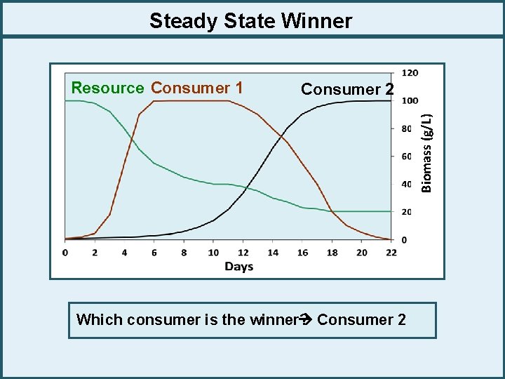
Steady State Winner Consumer 2 Biomass (g/L) Resource Consumer 1 Consumer 2 Which consumer is the winner?

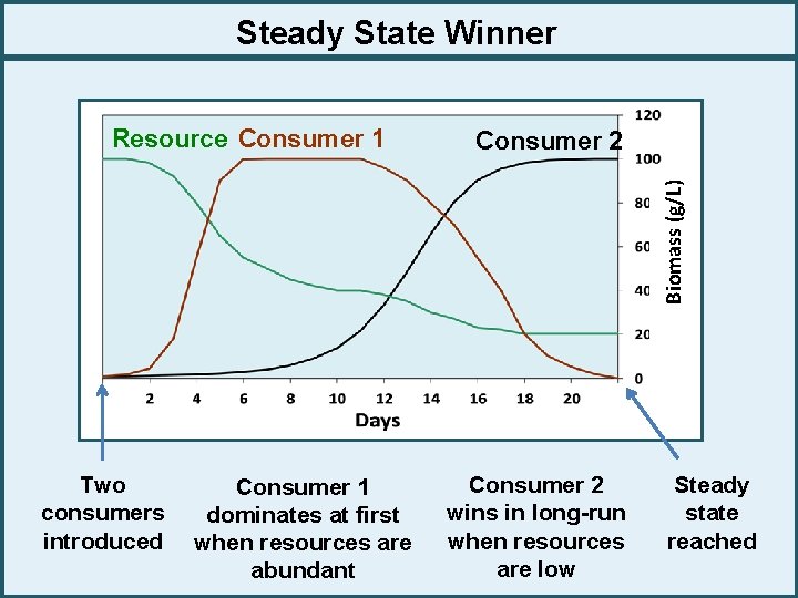
Steady State Winner Consumer 2 Biomass (g/L) Resource Consumer 1 Two consumers introduced Consumer 1 dominates at first when resources are abundant Consumer 2 wins in long-run when resources are low Steady state reached

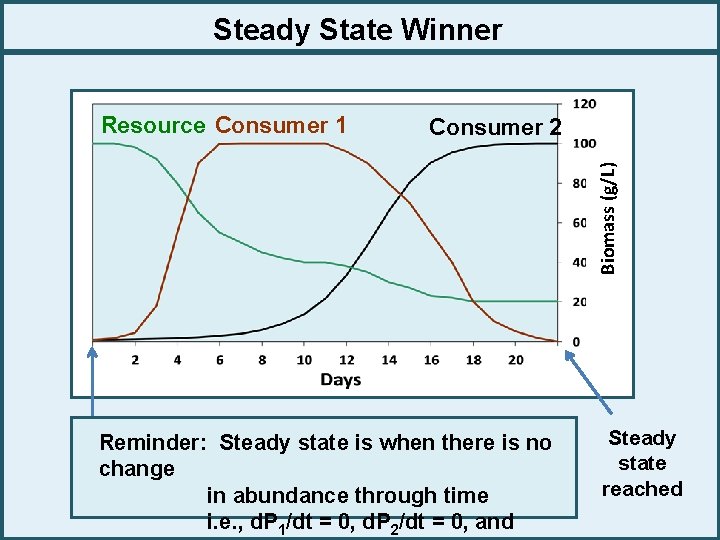
Steady State Winner Consumer 2 Biomass (g/L) Resource Consumer 1 Reminder: Steady state is when there is no change in abundance through time i. e. , d. P 1/dt = 0, d. P 2/dt = 0, and Steady state reached

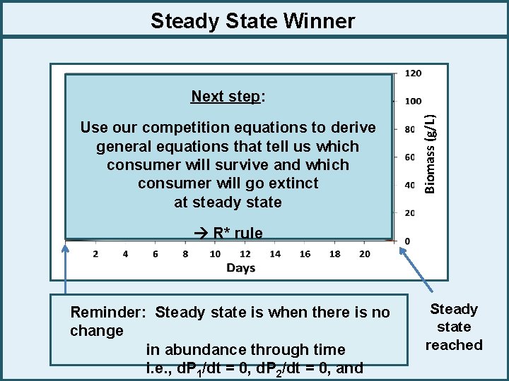
Steady State Winner Consumer Next 1 step: Consumer 2 Use our competition equations to derive general equations that tell us which consumer will survive and which consumer will go extinct at steady state Biomass (g/L) Resource R* rule Reminder: Steady state is when there is no change in abundance through time i. e. , d. P 1/dt = 0, d. P 2/dt = 0, and Steady state reached

R* Rule determines competitive dominance at steady state R* is the resource level at equilibrium The R* Rule: The resource abundance at equilibrium (R*) is that level of the resource at which the consumer is just maintained in the system i. e. , R* is the lowest resource level at which a consumer can be sustained If the resource level were to decrease, the consumer would go extinct à Each consumer has it’s own R* Competing consumers will (almost always) have different R* will determine which consumer wins

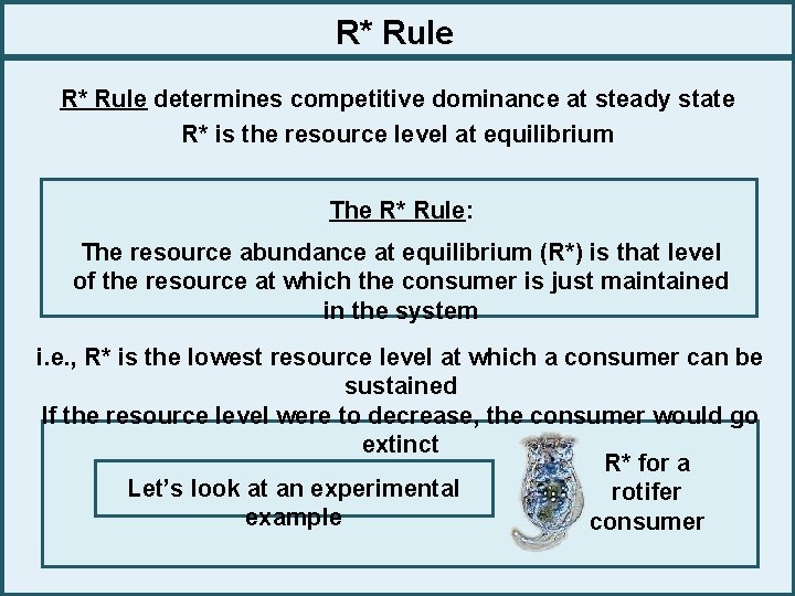
R* Rule determines competitive dominance at steady state R* is the resource level at equilibrium The R* Rule: The resource abundance at equilibrium (R*) is that level of the resource at which the consumer is just maintained in the system i. e. , R* is the lowest resource level at which a consumer can be sustained If the resource level were to decrease, the consumer would go extinct R* for a Let’s look at an experimental rotifer example consumer

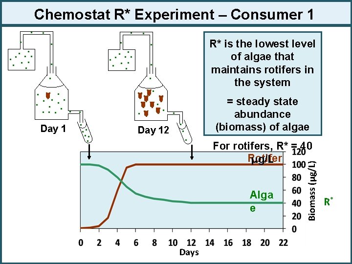
Chemostat R* Experiment – Consumer 1 . . Day 12 R* is the lowest level of algae that maintains rotifers in the system . . . = steady state abundance (biomass) of algae For rotifers, R* = 40 Rotifer μg/L Alga e Days Biomass (μg/L) . . . . Day 1. . . R*

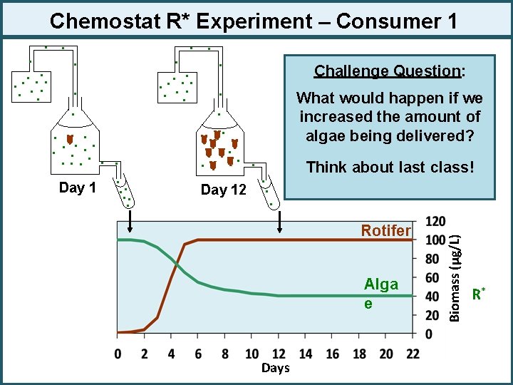
Chemostat R* Experiment – Consumer 1 . . Day 12 Challenge Question: What would happen if we increased the amount of algae being delivered? . . . Think about last class! Rotifer Alga e Days Biomass (μg/L) . . . . Day 1. . . R*

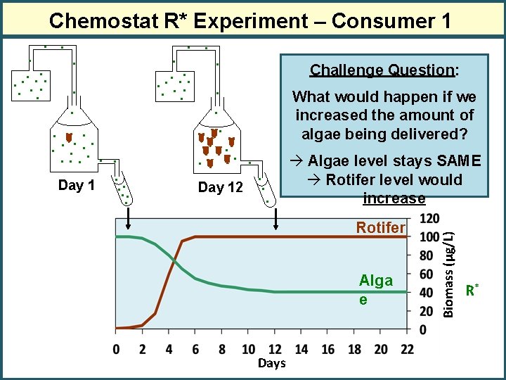
Chemostat R* Experiment – Consumer 1 . . Day 12 Challenge Question: What would happen if we increased the amount of algae being delivered? . . . à Algae level stays SAME à Rotifer level would increase Rotifer Alga e Days Biomass (μg/L) . . . . Day 1. . . R*

R* Rule That’s how we can determine R* empirically (experimentally) for a single species Can also determine R* by building an equation Let’s derive equation for R* Recall for predator-prey equations that we used the predator equation to derive equation for V* and prey equation to derive equation for P* Likewise, we will use consumer equation to derive equation for R* We’ll start with Consumer 1

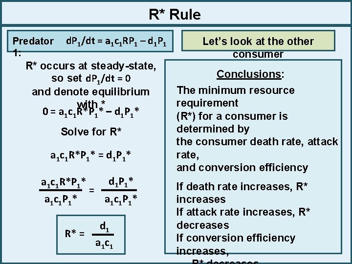
R* Rule Predator 1: d. P 1/dt = a 1 c 1 RP 1 – d 1 P 1 R* occurs at steady-state, so set d. P 1/dt = 0 and denote equilibrium with * 0 = a 1 c 1 R*P 1* – d 1 P 1* Solve for R* a 1 c 1 R*P 1* = d 1 P 1* a 1 c 1 R*P 1* a 1 c 1 P 1 * = d 1 P 1 * a 1 c 1 P 1 * d 1 R* = a 1 c 1 Let’s look at the other consumer Conclusions: The minimum resource requirement (R*) for a consumer is determined by the consumer death rate, attack rate, and conversion efficiency If death rate increases, R* increases If attack rate increases, R* decreases If conversion efficiency increases,

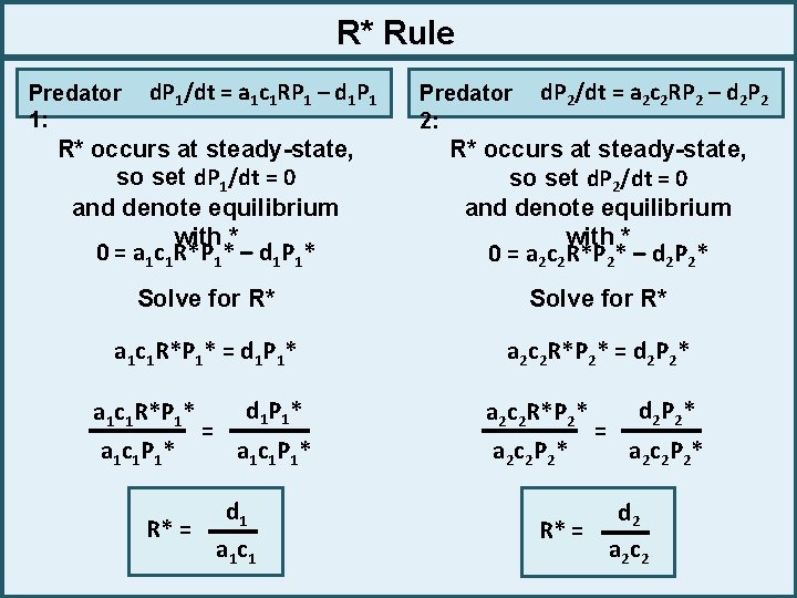
R* Rule Predator 1: d. P 1/dt = a 1 c 1 RP 1 – d 1 P 1 Predator 2: d. P 2/dt = a 2 c 2 RP 2 – d 2 P 2 R* occurs at steady-state, so set d. P 1/dt = 0 and denote equilibrium with * 0 = a 1 c 1 R*P 1* – d 1 P 1* R* occurs at steady-state, so set d. P 2/dt = 0 and denote equilibrium with * 0 = a 2 c 2 R*P 2* – d 2 P 2* Solve for R* a 1 c 1 R*P 1* = d 1 P 1* a 2 c 2 R*P 2* = d 2 P 2* a 1 c 1 R*P 1* a 1 c 1 P 1 * = d 1 P 1 * a 2 c 2 R*P 2* a 1 c 1 P 1 * a 2 c 2 P 2 * d 1 R* = a 1 c 1 = d 2 P 2 * a 2 c 2 P 2 * d 2 R* = a 2 c 2

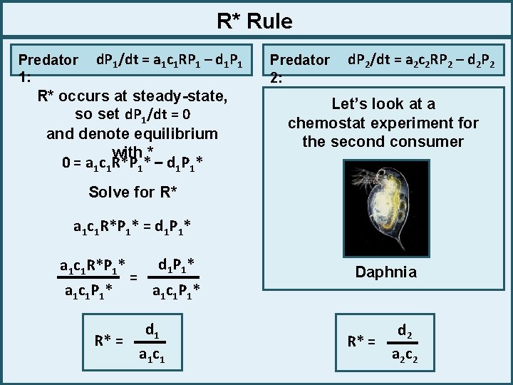
R* Rule Predator 1: d. P 1/dt = a 1 c 1 RP 1 – d 1 P 1 R* occurs at steady-state, so set d. P 1/dt = 0 and denote equilibrium with * 0 = a 1 c 1 R*P 1* – d 1 P 1* Predator 2: d. P 2/dt = a 2 c 2 RP 2 – d 2 P 2 Let’s look at a chemostat experiment for the second consumer Solve for R* a 1 c 1 R*P 1* = d 1 P 1* a 1 c 1 R*P 1* a 1 c 1 P 1 * = d 1 P 1 * a 1 c 1 P 1 * d 1 R* = a 1 c 1 Daphnia d 2 R* = a 2 c 2

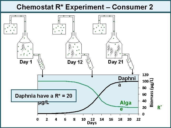
Chemostat R* Experiment – Consumer 2 . . . Day 21 Day 12. . . Daphni a Daphnia have a R* = 20 μg/L Alga e Days Biomass (μg/L) . . . . Day 1. . . R*

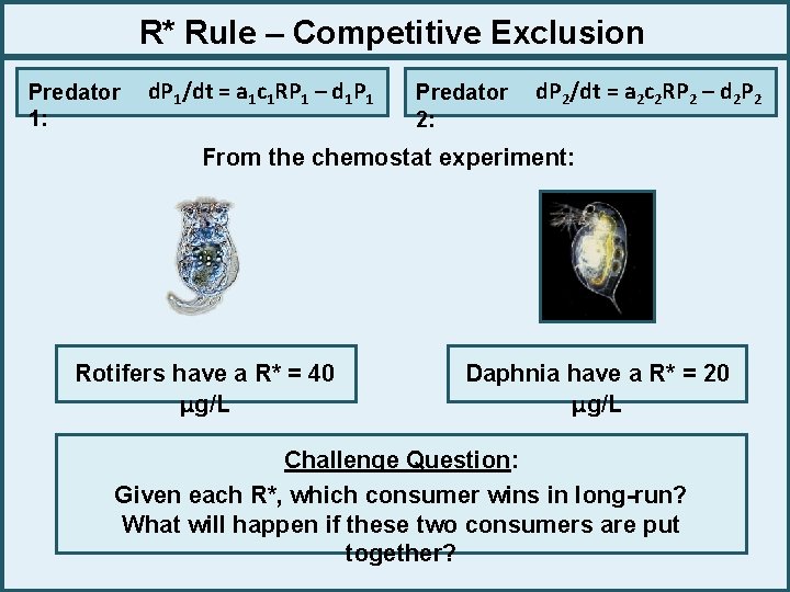
R* Rule – Competitive Exclusion Predator 1: d. P 1/dt = a 1 c 1 RP 1 – d 1 P 1 Predator 2: d. P 2/dt = a 2 c 2 RP 2 – d 2 P 2 From the chemostat experiment: Rotifers have a R* = 40 μg/L Daphnia have a R* = 20 μg/L Challenge Question: Given each R*, which consumer wins in long-run? What will happen if these two consumers are put together?

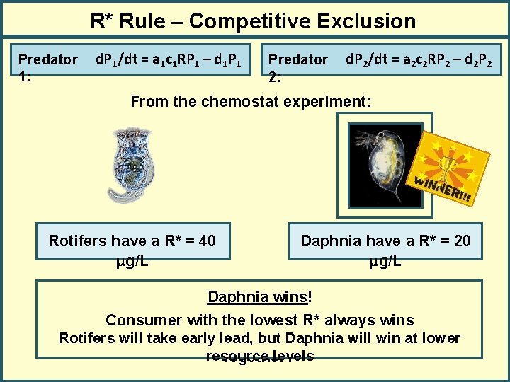
R* Rule – Competitive Exclusion Predator 1: d. P 1/dt = a 1 c 1 RP 1 – d 1 P 1 Predator 2: d. P 2/dt = a 2 c 2 RP 2 – d 2 P 2 From the chemostat experiment: Rotifers have a R* = 40 μg/L Daphnia have a R* = 20 μg/L Challenge Daphnia. Question: wins! Given each R*, with which consumer in long-run? Consumer the lowest R*wins always wins Rotifers earlyiflead, Daphnia will win lower What will take happen thesebut two consumers areatput resource levels together?

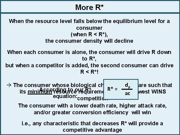
More R* When the resource level falls below the equilibrium level for a consumer (when R < R*), the consumer density will decline When each consumer is alone, the consumer will drive R down to R*, but when a competitor is added, the second consumer can drive R < R*! dp are such that à The consumer whose biological characteristics R* = According to our R* its minimum resource requirement (R*) are ac lowest WINS equation: competition The consumer with a lower death rate, higher attack rate, and/or greater conversion efficiency will win i. e. , any characteristic that decreases R* will provide a competitive advantage

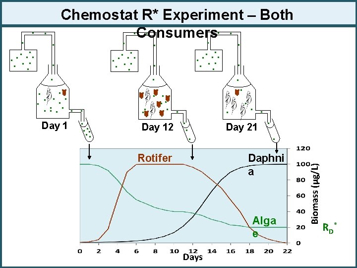
Chemostat R* Experiment – Both. . . Consumers. . . . . Day 12 . . . Rotifer . . . Day 21 . . . Daphni a Alga e Days Biomass (μg/L) . . R D*

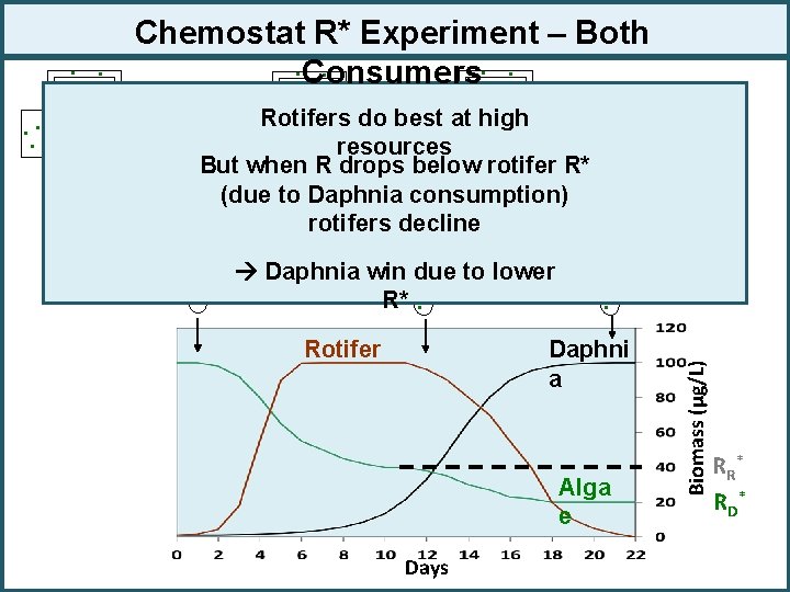
Chemostat R* Experiment – Both. . . Consumers. . . . high. . Rotifers do best at. . . . resources But when R. drops below rotifer. . R*. . consumption). (due to Daphnia. . . . rotifers. . . decline. . . win. . due to lower Day 1. . Daphnia Day 12 Day 21. . R*. . Rotifer Daphni a Alga e Days Biomass (μg/L) . . R R* R D*

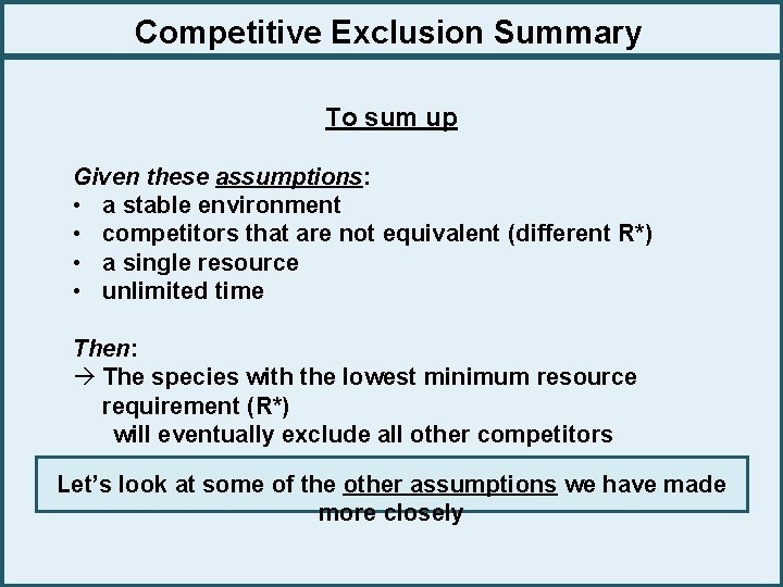
Competitive Exclusion Summary To sum up Given these assumptions: • a stable environment • competitors that are not equivalent (different R*) • a single resource • unlimited time Then: à The species with the lowest minimum resource requirement (R*) will eventually exclude all other competitors Let’s look at some of the other assumptions we have made more closely

Looking Ahead Next Class: More R* Adding Type II functional response Lab Tomorrow Competition modeling Stella lab – Meet in Computer Lab