Fundamentals of Statistics for Quality Control 1 Descriptive


 is a characteristic of a population, i. o. w. it")
ความแมนยำ และความถกตองของระบบวด ) True value Precision = a measure")


 • After sampling (collect data from production lot), data")
 Percentiles can be estimated from N")
![Skewness )ความเบ ( Negative skewed distribution Skew to the Left x[(n+1)/2] number )เลขค (](https://slidetodoc.com/presentation_image_h2/180522d4f15365012ad1473d865ab460/image-26.jpg "Skewness )ความเบ ( Negative skewed distribution Skew to the Left x[(n+1)/2] number )เลขค (")

 )กราฟทดสอบการแจกแจงแบบปกต ( Freq. Accumulative Freq. Normal distribution 50% 0 -1")

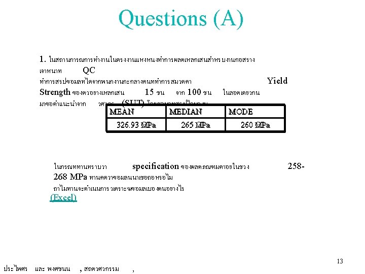
 ของหวบนทกขอมล (Magnetic Recording Head) แสดงไวดงน * (use Excel(")
- Slides: 32
Fundamentals of Statistics for Quality Control 1
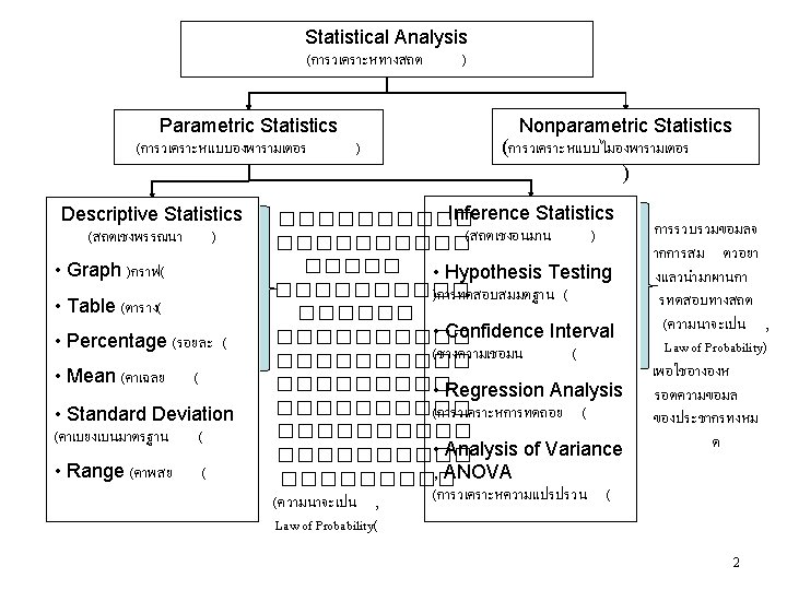
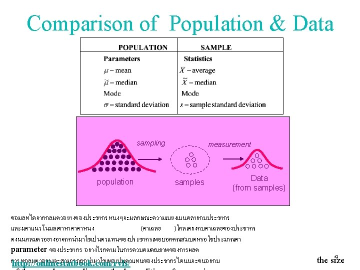
Descriptive and Inference Statistic ������ /measurement ����� Population Sample ������ � ������������ / ������ Sampling ���������� /inter pret Descriptive Statistics Population Sample ������� ������ / � ������ Sampling ����� /inter pret Conclusion ������� Inference Statistics 3
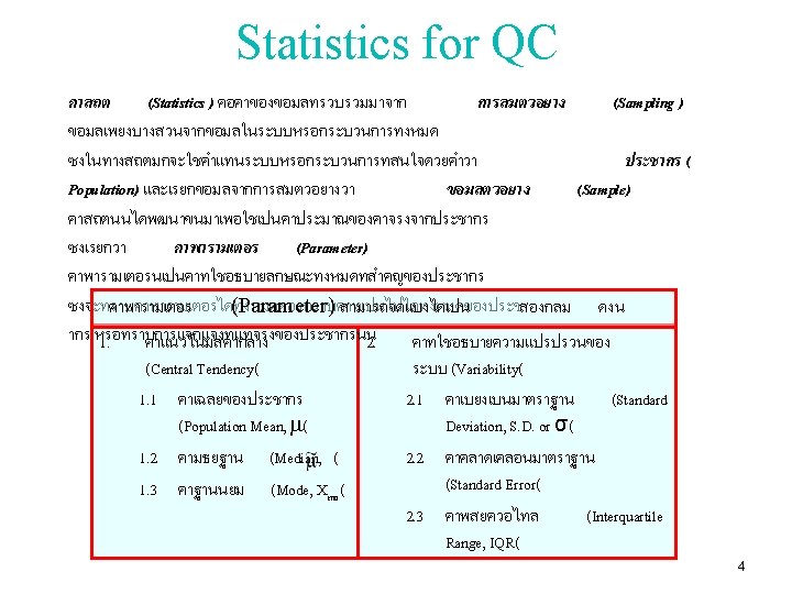
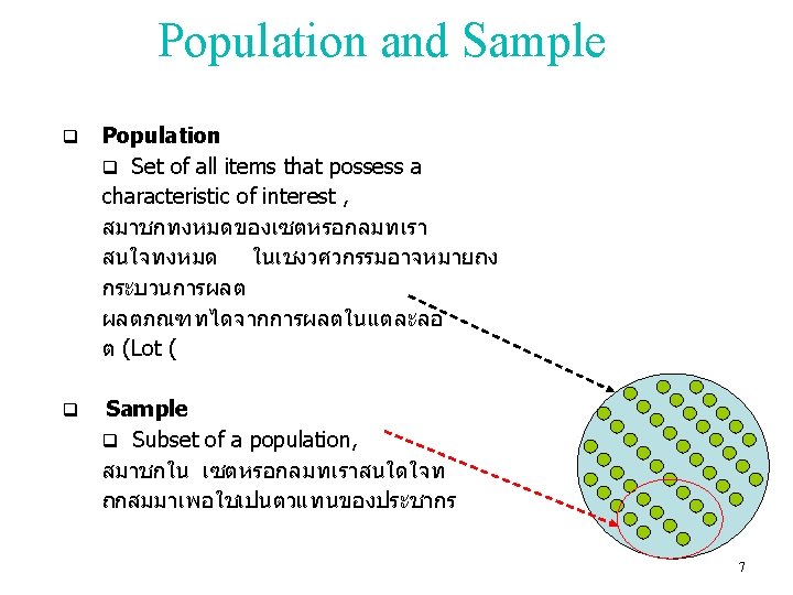
Parameter and Statistic Parameter(s) is a characteristic of a population, i. o. w. it describes a population , เปนคาทใชบรรยายลกษณะของประชากร เชน คาเฉลยของประชากร คาความแปรปรวนของประชากร q Example: average weight of the population, e. g. 50, 000 cans made in a month. Statistic(s) is a characteristic of a sample, used to make inferences on the population parameters that are typically unknown, called an estimator, เปนคาทใชบอกถงลกษณะของกลมตวอยางและคาเ หลานจะใชเพออนมาน หรอประมาณคา parameter ของประชากร q Example: average weight of a sample of 500 cans from that 8 month’s output, an estimate of the average weight of the
Precision and Accuracy of measurement system)ความแมนยำ และความถกตองของระบบวด ) True value Precision = a measure of the inherent variability in measurement system Accuracy = the ability of the instrument to measure the true value correctly on average High precision = Repeatability High accuracy= No Bias (small ε) bias Low precision = Low repeatability Accuracy = Bias (large ε) Low accuracy= Bias (small ε) Low precision = Low repeatability bias Low accuracy = Bias (large ε) 10
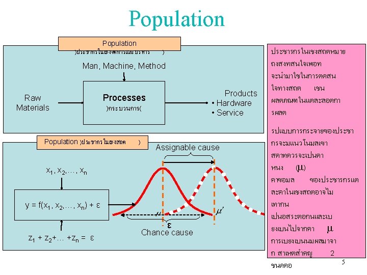
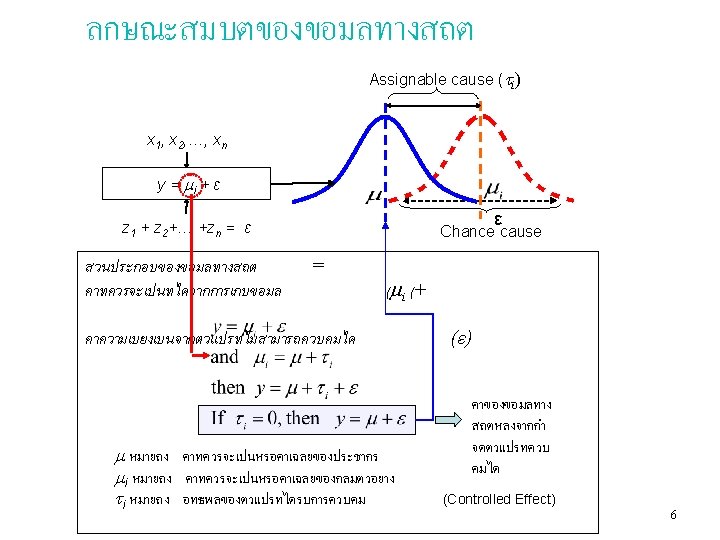
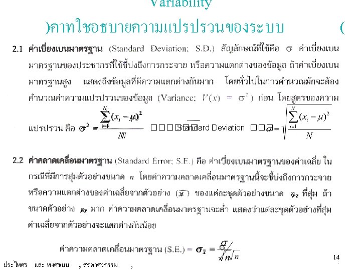
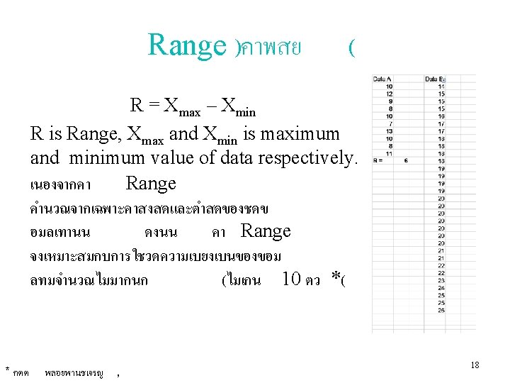
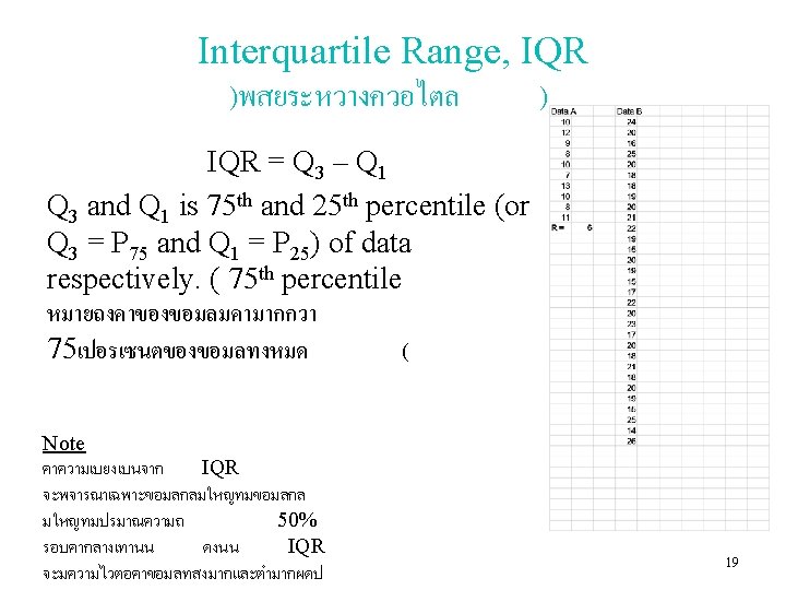
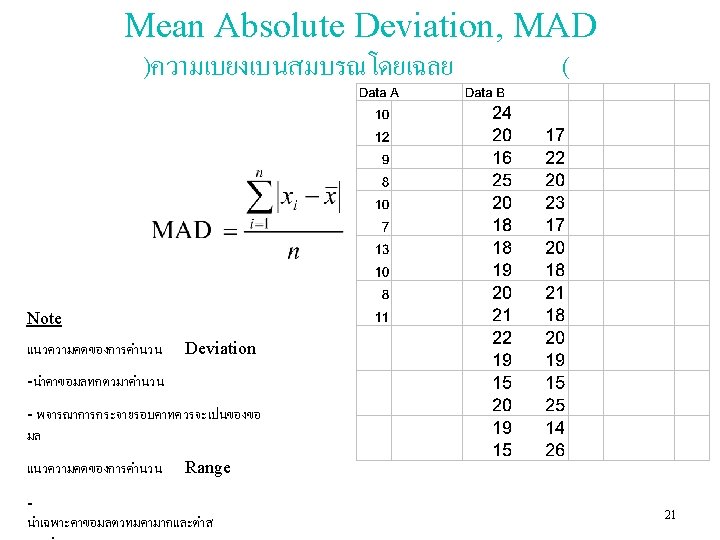
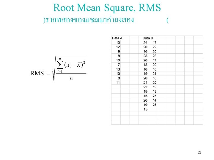
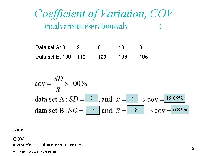
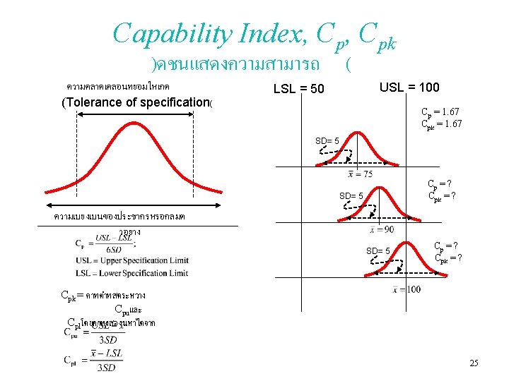
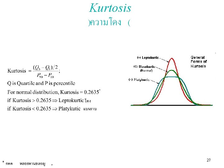
Statistical Data Analysis (for samples) • After sampling (collect data from production lot), data dispersion will be considered to evaluate the quality of data. หลงจากทำการสมตวอยางเกบขอมลจากลอตการผลต รปแบบการกระจายของขอมลจะถกนำมาประเมณคณภาพของขอมล • Data dispersion can be analyzed by using statistical parameters: – – – – Range Interquartile Range Mean Absolute Deviation Root Mean Square Standard deviation Coefficient of Variation Capability Index • In addition, data dispersion can be evaluated by considering the pattern of dispersion using – Skewness – Kurtosis – Normal Probability Paper (NOPP) 17
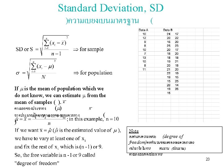
Supplement for percentile calculation Estimation of percentiles (1) Percentiles can be estimated from N measurements as follows: for the pth percentile, set p(N+1) equal to k + d for k an integer )เลขจำนวนเตม ), and d) ทศนยม ), a fraction greater than or equal to 0 and less than 1. example 1. For 0 < k < N, Y(p) = Y[k] + d(Y[k+1] - Y[k]); โดย Y(p) คอคาขอมลท Percentile ท p, และY[k] คอคาขอมลท Percentile ท k 2. For k = 0, Y(p) = Y[1] 3. For k = N, Y(p) = Y[N] (2) Some software packages (EXCEL, for example) set 1+p(N-1) equal to k + d, then proceed as above. )วธการคำนวณคา Percentile ของ EXCEL( (3) A third way of calculating percentiles starts by calculating p. N) p คณ N(. If p. N is not an integer )เลขจำนวนเตม ), round up )ปดคาทศนยมขนเปนจำนวนเตม ) to the next highest integer k and , percentile Y(p) = Y[k] as the percentile estimate. If p. N is an integer k, 20
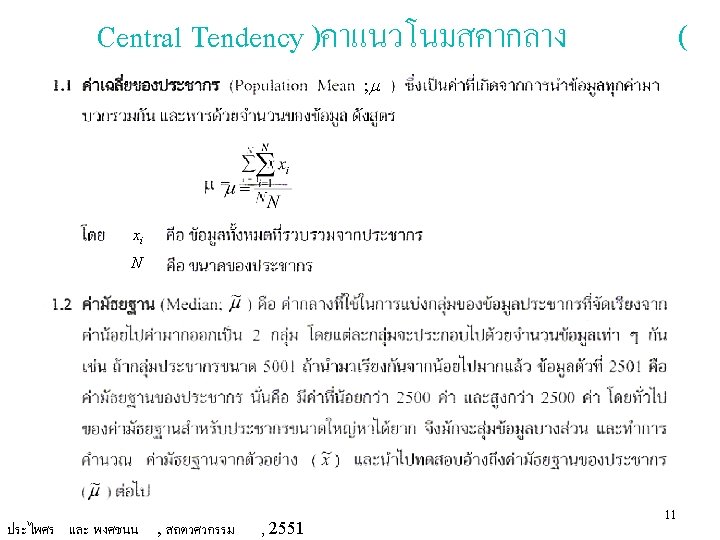
Skewness )ความเบ ( Negative skewed distribution Skew to the Left x[(n+1)/2] number )เลขค ( (x(n/2) + y(n/2)+1)/2 )เลขค ( if n is an odd if n is an even number Normal distribution xn หมายถงคาของขอ มลลำดบท n Positive skewed distribution Skew to the Right 26
Normal Probability Paper (NOPP) )กราฟทดสอบการแจกแจงแบบปกต ( Freq. Accumulative Freq. Normal distribution 50% 0 -1 -2 -3 0 1 2 3 -1 -2 -3 0 1 2 How to plot a graph on NOPP 3 1. Rearrange the data in ascending or descending order )จดเรยงขอมลตามลำดบนอยไปหามากหรอมากไปนอยกได ( 2. Calculate accumulative percentage by using this equation: )หาคาเปอรเซนตหรอความถสะสม ( 3. Use the data to plot the curve on NOPP) สรางกราฟบน NOPP( 4. If the plotting result is a straight line, data dispersion is normal distribution )ถากราฟทไดปนเสนตรงแสดงวาขอมลมการแจกแจงแบบปกต ) 30
การใช NOPP สำหรบขอมลจำนวนนอย ในการศกษาถงความสามารถในการวดซำ หรอ Repeatability (ซงเปนสวนหนงของ Gauge Repeatability & Reproducibility or Gauge R&R ( ของเพลาชนหนงซงมเสนผานศนยกลาง ซ. ม. ไดผลดงน Excel to prepare( (use 10. 19. 6 10. 010. 210. 39. 59. 79. 810. 2 ใหพจารณาวาขอมลทไดดงกลาวมการแจงแบบปกตหรอไม ถาใช ทานคดวาระบบการวดนนาเชอถอไดหรอไม ถาไม อะไรททานคดวานาจะเปนสาเหต Note: There are two important aspects on a Gauge R&R: Repeatability, Repeatability is the variation in measurements taken by a single person or instrument on the same item and under the same conditions. Reproducibility, the variability induced by the operators. It is the variation induced when different operators 31 (or different laboratories) measure the same part.
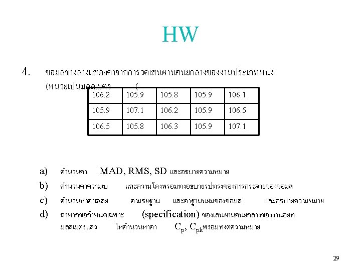
การใช NOPP สำหรบขอมลจำนวนมาก ขอมลจากการวดความกวางของชองวาง (Gap Width) ของหวบนทกขอมล (Magnetic Recording Head) แสดงไวดงน * (use Excel( * กตต พลอยพานชเจรญ 1. 39 1. 40 1. 60 1. 41 1. 43 1. 46 1. 30 1. 50 1. 34 1. 47 1. 56 1. 35 1. 52 1. 51 1. 25 1. 39 1. 55 1. 59 1. 50 1. 66 1. 61 1. 32 1. 46 1. 30 1. 51 1. 52 1. 48 1. 38 1. 40 1. 55 1. 39 1. 33 1. 46 1. 43 1. 35 1. 57 1. 50 1. 20 1. 48 1. 41 1. 65 1. 51 1. 42 1. 60 1. 29 1. 38 1. 46 1. 39 1. 42 1. 46 1. 69 1. 55 1. 46 1. 52 1. 33 1. 52 1. 25 1. 48 1. 60 1. 43 1. 51 1. 35 1. 40 1. 46 1. 57 1. 62 1. 46 1. 51 1. 24 1. 50 1. 56 1. 30 1. 40 1. 55 1. 50 1. 52 1. 43 1. 39 1. 41 1. 38 1. 40 1. 35 1. 48 1. 42 1. 30 1. 38 1. 55 1. 46 1. 58 1. 34 1. 41 1. 29 1. 41 1. 42 1. 43 1. 38 1. 42 1. 60 1. 35 , 32