Fundamentals of Real Estate Lecture 12 Spring 2003

Fundamentals of Real Estate Lecture 12 Spring, 2003 Copyright © Joseph A. Petry www. cba. uiuc. edu/jpetry/Fin_264_sp 03

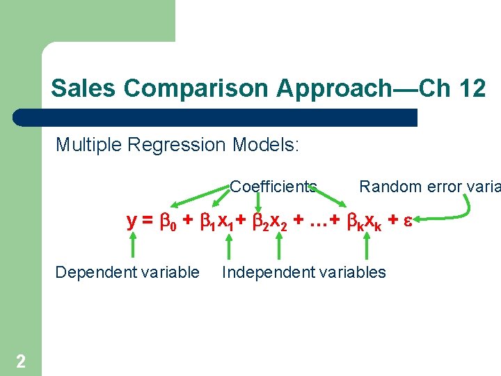
Sales Comparison Approach—Ch 12 Multiple Regression Models: Coefficients Random error varia y = b 0 + b 1 x 1+ b 2 x 2 + …+ bkxk + e Dependent variable 2 Independent variables

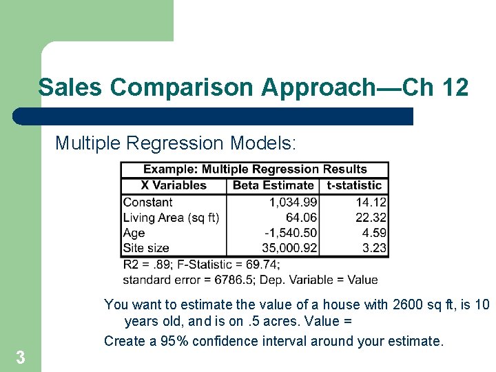
Sales Comparison Approach—Ch 12 Multiple Regression Models: 3 You want to estimate the value of a house with 2600 sq ft, is 10 years old, and is on. 5 acres. Value = Create a 95% confidence interval around your estimate.

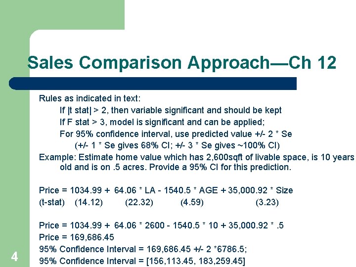
Sales Comparison Approach—Ch 12 Rules as indicated in text: If |t stat| > 2, then variable significant and should be kept If F stat > 3, model is significant and can be applied; For 95% confidence interval, use predicted value +/- 2 * Se (+/- 1 * Se gives 68% CI; +/- 3 * Se gives ~100% CI) Example: Estimate home value which has 2, 600 sqft of livable space, is 10 years old and is on. 5 acres. Provide a 95% CI for this prediction. Price = 1034. 99 + 64. 06 * LA - 1540. 5 * AGE + 35, 000. 92 * Size (t-stat) (14. 12) (22. 32) (4. 59) (3. 23) 4 Price = 1034. 99 + 64. 06 * 2600 - 1540. 5 * 10 + 35, 000. 92 *. 5 Price = 169, 686. 45 95% Confidence Interval = 169, 686. 45 +/- 2 *6786. 5; 95% Confidence Interval = [156, 113. 45, 183, 259. 45]

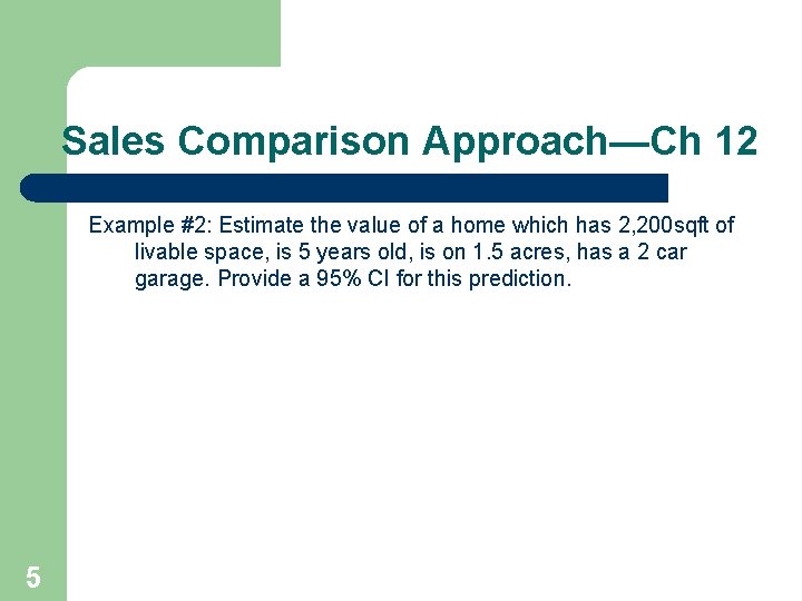
Sales Comparison Approach—Ch 12 Example #2: Estimate the value of a home which has 2, 200 sqft of livable space, is 5 years old, is on 1. 5 acres, has a 2 car garage. Provide a 95% CI for this prediction. 5

Project Description You and your team members are interested in investing in some apartment buildings in Champaign-Urbana. Each team will have narrowed down their choices to a few investment opportunities, along with brief information about the current owners. Your objective in the project is to: 1. 2. 3. 6 Use the market data that your team has already collected to obtain solid estimates of the income potential of each property. This should be done relying on a well-specified multiple regression model. Analyze each investment opportunity using the tools developed in this class. To the extent you have expense data available for the property, you can use it. Otherwise, you will have to depend on reasonable estimates. Establish the highest purchase price that you would be willing to pay for each property. Develop a strategy of which property to pursue, at what price and for how long. Develop a similar strategy for the second property.

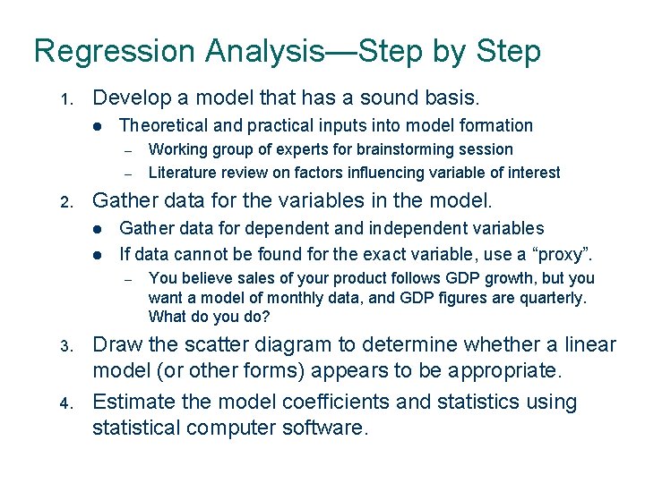
Regression Analysis—Step by Step 1. Develop a model that has a sound basis. l Theoretical and practical inputs into model formation – – 2. Gather data for the variables in the model. l l Gather data for dependent and independent variables If data cannot be found for the exact variable, use a “proxy”. – 3. 4. 7 Working group of experts for brainstorming session Literature review on factors influencing variable of interest You believe sales of your product follows GDP growth, but you want a model of monthly data, and GDP figures are quarterly. What do you do? Draw the scatter diagram to determine whether a linear model (or other forms) appears to be appropriate. Estimate the model coefficients and statistics using statistical computer software.

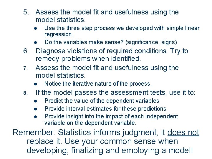
5. Assess the model fit and usefulness using the model statistics. l l Use three step process we developed with simple linear regression. Do the variables make sense? (significance, signs) 6. Diagnose violations of required conditions. Try to remedy problems when identified. 7. Assess the model fit and usefulness using the model statistics. l 8. Notice the iterative nature of the process. If the model passes the assessment tests, use it to: l l l Predict the value of the dependent variables Provide interval estimates for these predictions Provide insight into the impact of each independent variable on the dependent variable. Remember: Statistics informs judgment, it does not replace it. Use your common sense when developing, finalizing and employing a model! 8

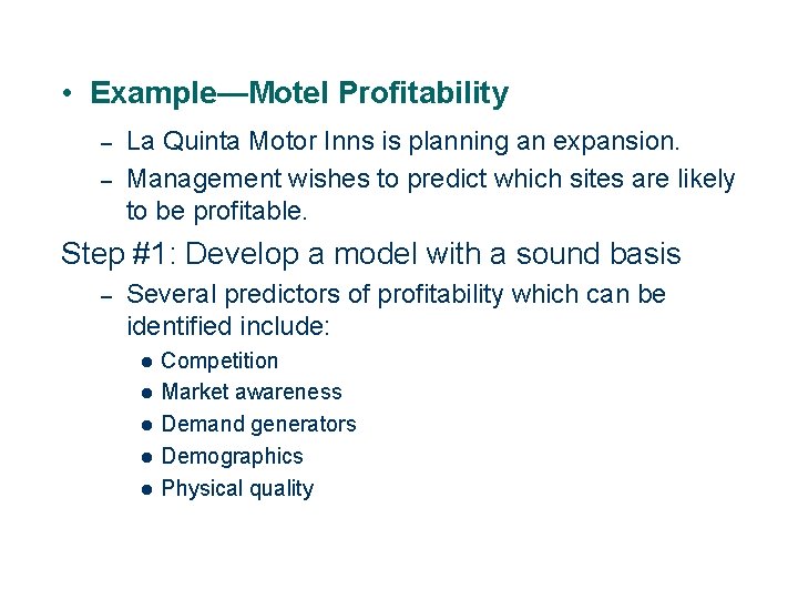
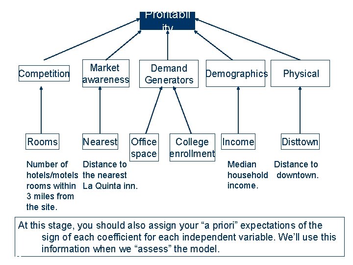
• Example—Motel Profitability – – La Quinta Motor Inns is planning an expansion. Management wishes to predict which sites are likely to be profitable. Step #1: Develop a model with a sound basis – Several predictors of profitability which can be identified include: l l l 9 Competition Market awareness Demand generators Demographics Physical quality

Profitabil ity Competition Rooms Market awareness Nearest Demand Generators Office space Distance to Number of hotels/motels the nearest rooms within La Quinta inn. 3 miles from the site. Demographics College Income enrollment Physical Disttown Median Distance to household downtown. income. At this stage, you should also assign your “a priori” expectations of the sign of each coefficient for each independent variable. We’ll use this information when we “assess” the model. 10

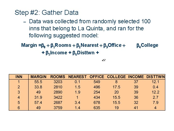
Step #2: Gather Data – Data was collected from randomly selected 100 inns that belong to La Quinta, and ran for the following suggested model: Margin =b 0 + b 1 Rooms + b 2 Nearest + b 3 Office + + b 5 Income + b 6 Disttwn + 11 b 4 College

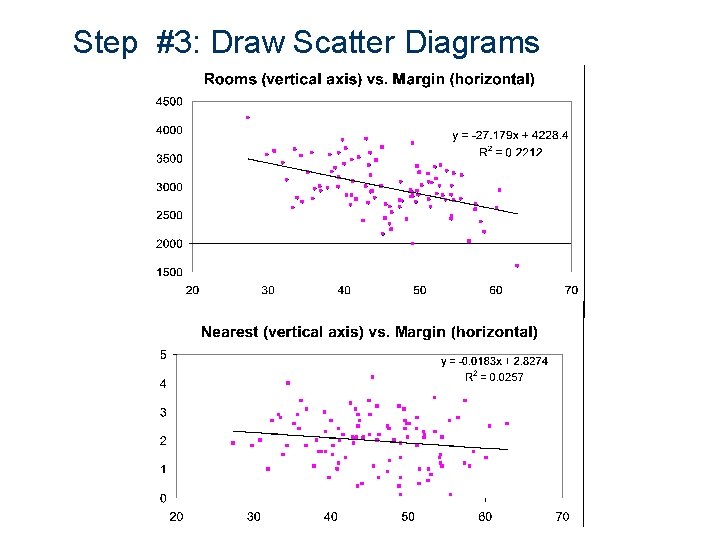
Step #3: Draw Scatter Diagrams 12

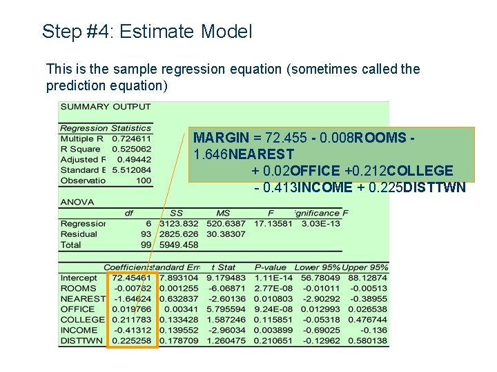
Step #4: Estimate Model This is the sample regression equation (sometimes called the prediction equation) MARGIN = 72. 455 - 0. 008 ROOMS 1. 646 NEAREST + 0. 02 OFFICE +0. 212 COLLEGE - 0. 413 INCOME + 0. 225 DISTTWN 13

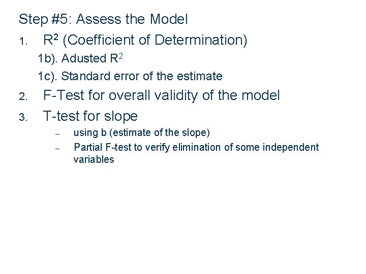
Step #5: Assess the Model 1. R 2 (Coefficient of Determination) 1 b). Adusted R 2 1 c). Standard error of the estimate 2. 3. F-Test for overall validity of the model T-test for slope – – 14 using b (estimate of the slope) Partial F-test to verify elimination of some independent variables

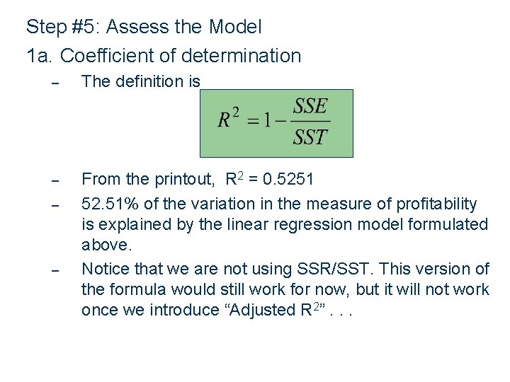
Step #5: Assess the Model 1 a. Coefficient of determination – The definition is – From the printout, R 2 = 0. 5251 52. 51% of the variation in the measure of profitability is explained by the linear regression model formulated above. Notice that we are not using SSR/SST. This version of the formula would still work for now, but it will not work once we introduce “Adjusted R 2”. . . – – 15

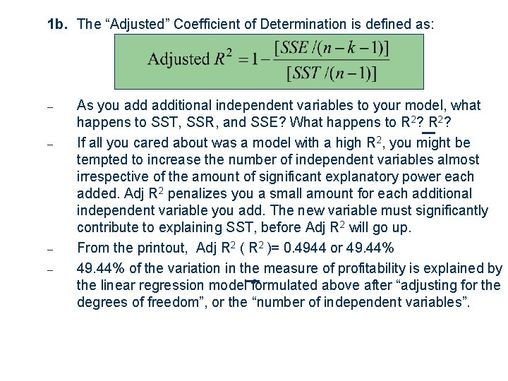
1 b. The “Adjusted” Coefficient of Determination is defined as: – – 16 As you additional independent variables to your model, what happens to SST, SSR, and SSE? What happens to R 2? If all you cared about was a model with a high R 2, you might be tempted to increase the number of independent variables almost irrespective of the amount of significant explanatory power each added. Adj R 2 penalizes you a small amount for each additional independent variable you add. The new variable must significantly contribute to explaining SST, before Adj R 2 will go up. From the printout, Adj R 2 ( R 2 )= 0. 4944 or 49. 44% of the variation in the measure of profitability is explained by the linear regression model formulated above after “adjusting for the degrees of freedom”, or the “number of independent variables”.

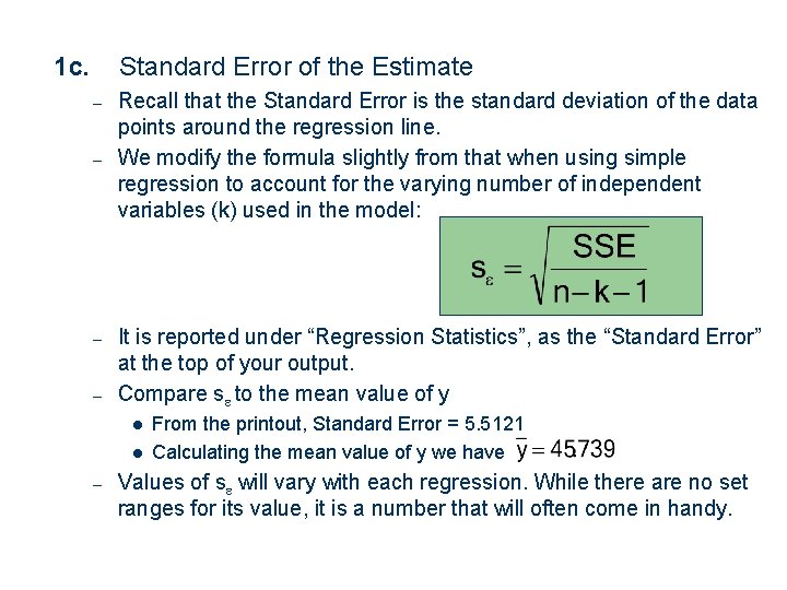
1 c. Standard Error of the Estimate – – Recall that the Standard Error is the standard deviation of the data points around the regression line. We modify the formula slightly from that when using simple regression to account for the varying number of independent variables (k) used in the model: It is reported under “Regression Statistics”, as the “Standard Error” at the top of your output. Compare se to the mean value of y l l – 17 From the printout, Standard Error = 5. 5121 Calculating the mean value of y we have Values of se will vary with each regression. While there are no set ranges for its value, it is a number that will often come in handy.

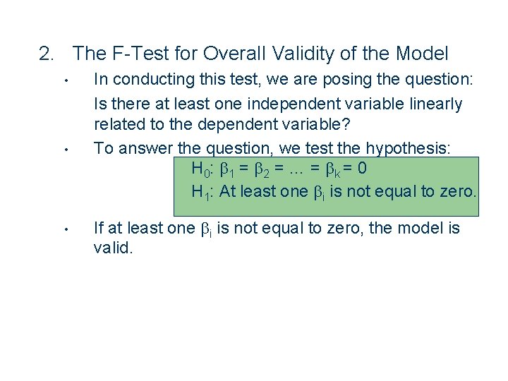
2. The F-Test for Overall Validity of the Model • • • 18 In conducting this test, we are posing the question: Is there at least one independent variable linearly related to the dependent variable? To answer the question, we test the hypothesis: H 0: b 1 = b 2 = … = b k = 0 H 1: At least one bi is not equal to zero. If at least one bi is not equal to zero, the model is valid.

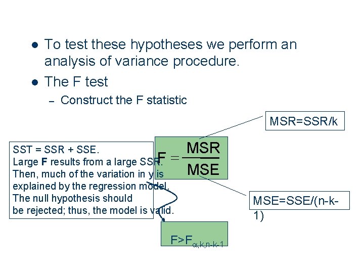
l l To test these hypotheses we perform an analysis of variance procedure. The F test – Construct the F statistic MSR=SSR/k SST = SSR + SSE. F= Large F results from a large SSR. Then, much of the variation in y is explained the regression model. – by Rejection region The null hypothesis should be rejected; thus, the model is valid. MSR MSE F>Fa, k, n-k-1 19 MSE=SSE/(n-k 1)

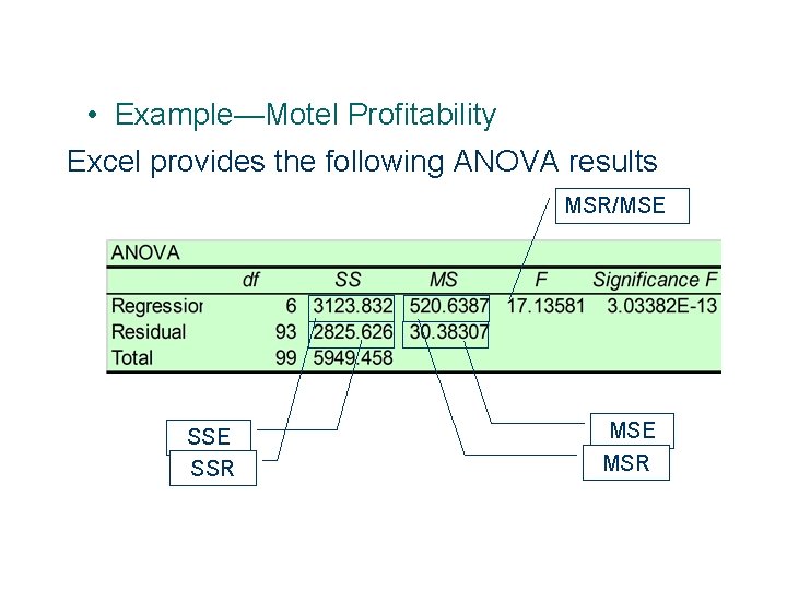
• Example—Motel Profitability Excel provides the following ANOVA results MSR/MSE SSR 20 MSE MSR

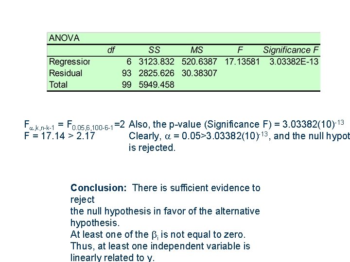
Fa, k, n-k-1 = F 0. 05, 6, 100 -6 -1=2. 17 Also, the p-value (Significance F) = 3. 03382(10)-13 F = 17. 14 > 2. 17 Clearly, a = 0. 05>3. 03382(10)-13, and the null hypot is rejected. 21 Conclusion: There is sufficient evidence to reject the null hypothesis in favor of the alternative hypothesis. At least one of the bi is not equal to zero. Thus, at least one independent variable is linearly related to y.

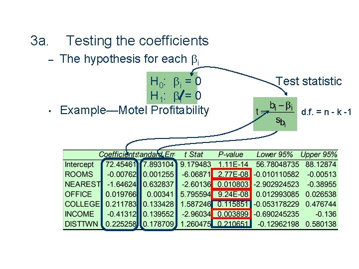
3 a. 22 Testing the coefficients – The hypothesis for each bi • H 0: b i = 0 H 1: b i = 0 Example—Motel Profitability Test statistic d. f. = n - k -1

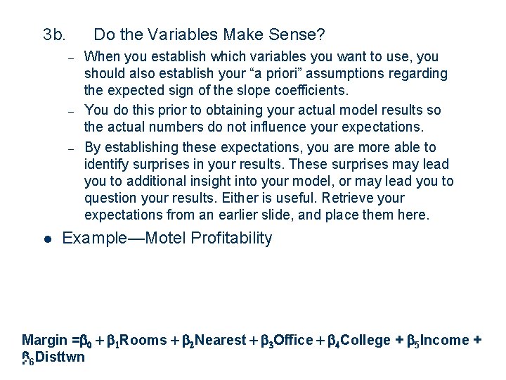
3 b. Do the Variables Make Sense? – – – l When you establish which variables you want to use, you should also establish your “a priori” assumptions regarding the expected sign of the slope coefficients. You do this prior to obtaining your actual model results so the actual numbers do not influence your expectations. By establishing these expectations, you are more able to identify surprises in your results. These surprises may lead you to additional insight into your model, or may lead you to question your results. Either is useful. Retrieve your expectations from an earlier slide, and place them here. Example—Motel Profitability Margin =b 0 + b 1 Rooms + b 2 Nearest + b 3 Office + b 4 College + b 5 Income + b 6 Disttwn 23

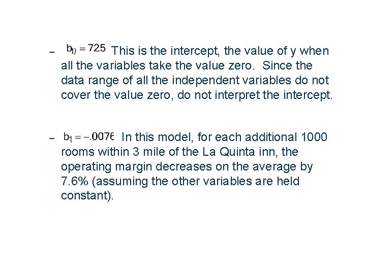
24 – This is the intercept, the value of y when all the variables take the value zero. Since the data range of all the independent variables do not cover the value zero, do not interpret the intercept. – In this model, for each additional 1000 rooms within 3 mile of the La Quinta inn, the operating margin decreases on the average by 7. 6% (assuming the other variables are held constant).

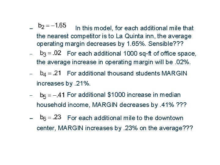
– In this model, for each additional mile that the nearest competitor is to La Quinta inn, the average operating margin decreases by 1. 65%. Sensible? ? ? – For each additional 1000 sq-ft of office space, the average increase in operating margin will be. 02%. – For additional thousand students MARGIN increases by. 21%. – For additional $1000 increase in median household income, MARGIN decreases by. 41% ? ? ? – For each additional mile to the downtown center, MARGIN increases by. 23% on the average? ? ? 25

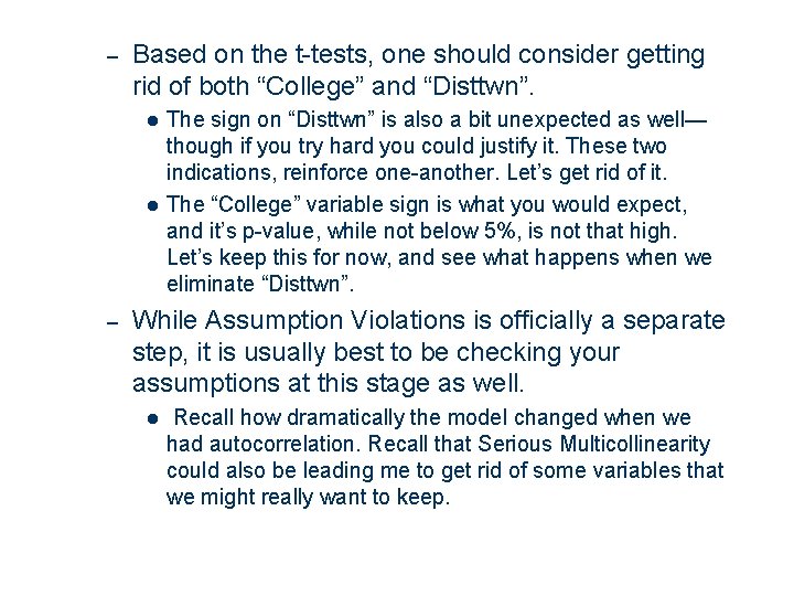
– Based on the t-tests, one should consider getting rid of both “College” and “Disttwn”. l l – While Assumption Violations is officially a separate step, it is usually best to be checking your assumptions at this stage as well. l 26 The sign on “Disttwn” is also a bit unexpected as well— though if you try hard you could justify it. These two indications, reinforce one-another. Let’s get rid of it. The “College” variable sign is what you would expect, and it’s p-value, while not below 5%, is not that high. Let’s keep this for now, and see what happens when we eliminate “Disttwn”. Recall how dramatically the model changed when we had autocorrelation. Recall that Serious Multicollinearity could also be leading me to get rid of some variables that we might really want to keep.

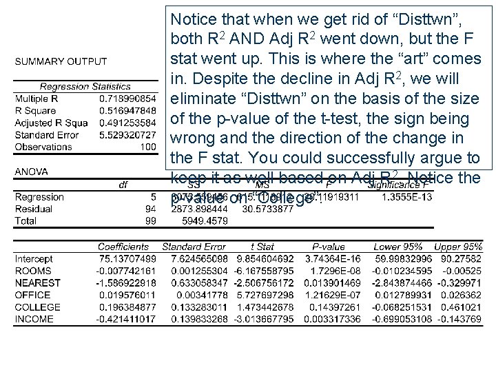
Notice that when we get rid of “Disttwn”, both R 2 AND Adj R 2 went down, but the F stat went up. This is where the “art” comes in. Despite the decline in Adj R 2, we will eliminate “Disttwn” on the basis of the size of the p-value of the t-test, the sign being wrong and the direction of the change in the F stat. You could successfully argue to keep it as well based on Adj R 2. Notice the p-value on “College”. 27

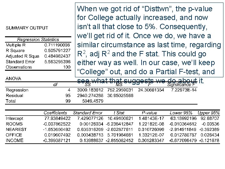
When we got rid of “Disttwn”, the p-value for College actually increased, and now isn’t all that close to 5%. Consequently, we’ll get rid of it. Once we do, we have a similar circumstance as last time, regarding R 2, adj R 2 and the F stat. This could go either way as well. In our case, we’ll keep “College” out, and do a Partial F-test, and see what that suggests we do about it. 28

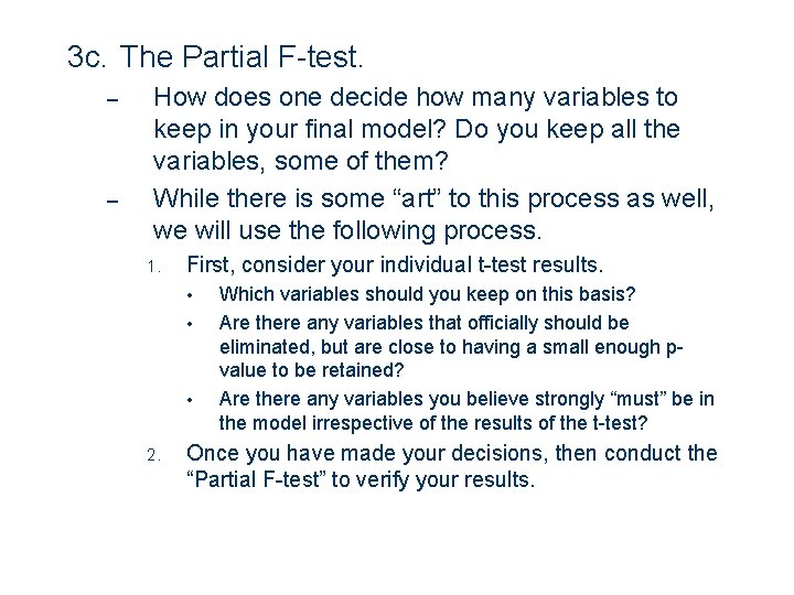
3 c. The Partial F-test. – – How does one decide how many variables to keep in your final model? Do you keep all the variables, some of them? While there is some “art” to this process as well, we will use the following process. 1. First, consider your individual t-test results. • • • 2. 29 Which variables should you keep on this basis? Are there any variables that officially should be eliminated, but are close to having a small enough pvalue to be retained? Are there any variables you believe strongly “must” be in the model irrespective of the results of the t-test? Once you have made your decisions, then conduct the “Partial F-test” to verify your results.

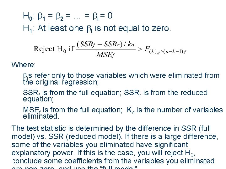
H 0: b 1 = b 2 = … = b i = 0 H 1: At least one bi is not equal to zero. Where: bis refer only to those variables which were eliminated from the original regression; SSRf is from the full equation; SSRr is from the reduced equation; MSEf is from the full equation; Kd is the number of variables eliminated. The test statistic is determined by the difference in SSR (full model) vs. SSR (reduced model). If there is a large difference, some of the variables you eliminated have significant explanatory power. If this is the case, you will reject H 0, 30 conclude some coefficients from the variables you eliminated

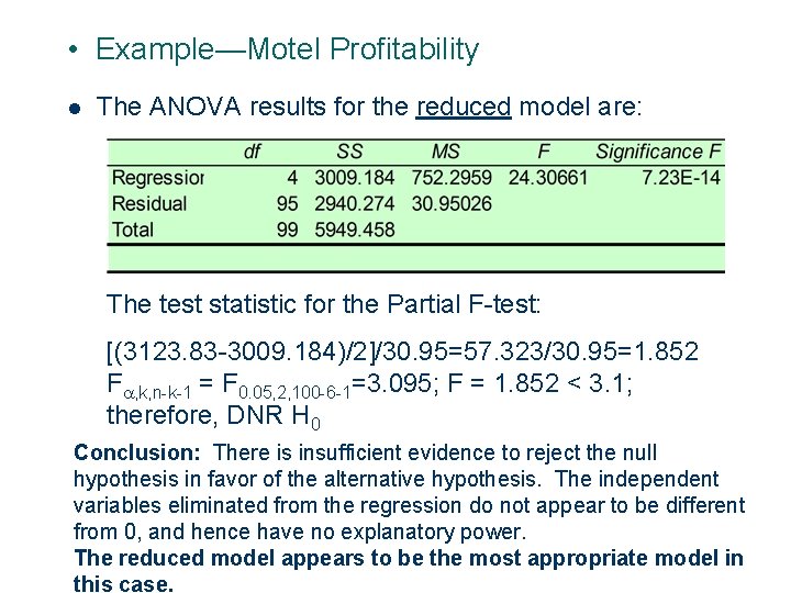
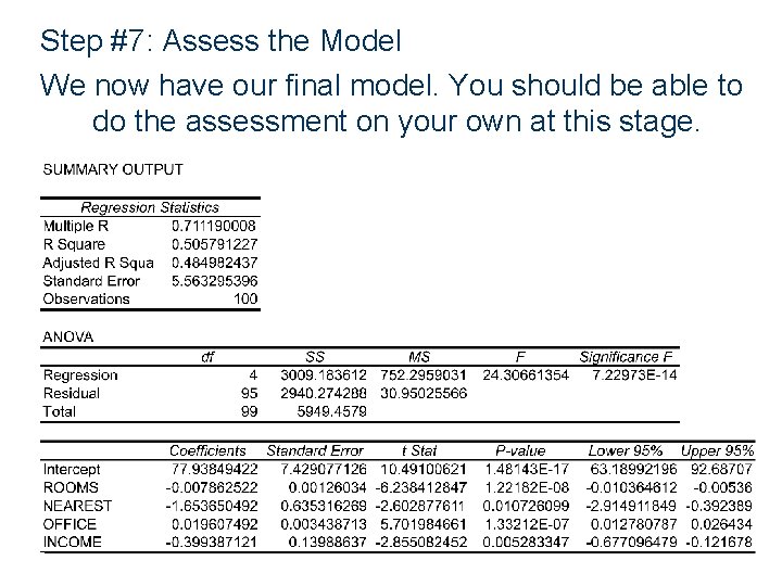
• Example—Motel Profitability l The ANOVA results for the reduced model are: The test statistic for the Partial F-test: [(3123. 83 -3009. 184)/2]/30. 95=57. 323/30. 95=1. 852 Fa, k, n-k-1 = F 0. 05, 2, 100 -6 -1=3. 095; F = 1. 852 < 3. 1; therefore, DNR H 0 31 Conclusion: There is insufficient evidence to reject the null hypothesis in favor of the alternative hypothesis. The independent variables eliminated from the regression do not appear to be different from 0, and hence have no explanatory power. The reduced model appears to be the most appropriate model in this case.

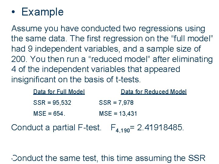
• Example Assume you have conducted two regressions using the same data. The first regression on the “full model” had 9 independent variables, and a sample size of 200. You then run a “reduced model” after eliminating 4 of the independent variables that appeared insignificant on the basis of t-tests. Data for Full Model Data for Reduced Model SSR = 95, 532 SSR = 7, 978 MSE = 654. MSE = 13, 431 Conduct a partial F-test. F 4, 190= 2. 41918485. 32 Conduct the same test, this time assuming the SSR

Step #6: Diagnose Violations of Required Conditions – – – 33 We already did this in concert with Step #5, and that is the way you really should do it. You cannot effectively assess the model, without having considered whether the assumptions have been violated. We separate them into steps only because both are so critical to constructing a useful regression model. Having to combine these critical steps is another manner in which the “art” of regression analysis becomes obvious.

Step #7: Assess the Model We now have our final model. You should be able to do the assessment on your own at this stage. 34

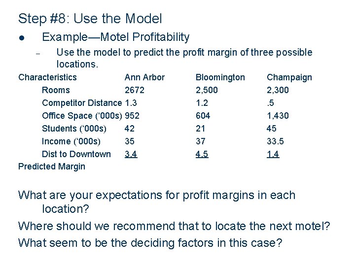
Step #8: Use the Model Example—Motel Profitability l – Use the model to predict the profit margin of three possible locations. Characteristics Ann Arbor Rooms 2672 Competitor Distance 1. 3 Office Space (‘ 000 s) 952 Students (‘ 000 s) 42 Income (‘ 000 s) 35 Dist to Downtown 3. 4 Predicted Margin Bloomington 2, 500 1. 2 604 21 37 4. 5 Champaign 2, 300. 5 1, 430 45 33. 5 1. 4 What are your expectations for profit margins in each location? Where should we recommend that to locate the next motel? What seem to be the deciding factors in this case? 35

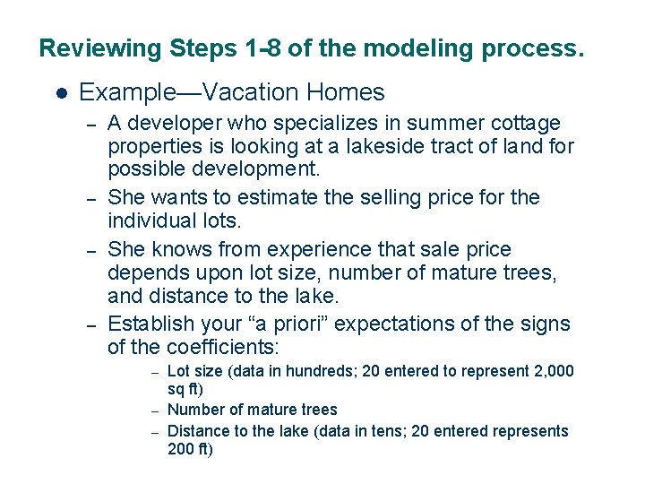
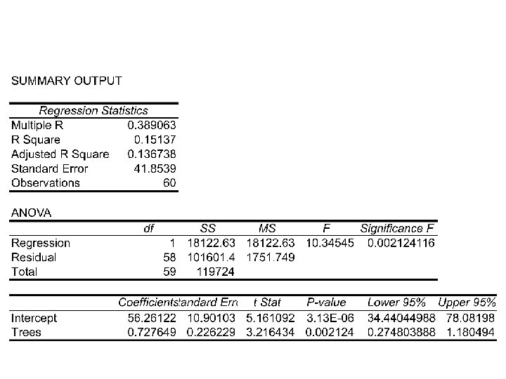
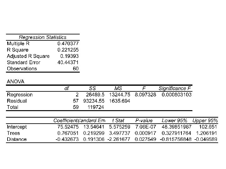
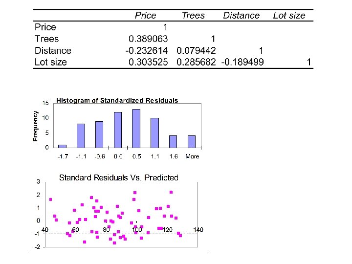
Reviewing Steps 1 -8 of the modeling process. l Example—Vacation Homes – – A developer who specializes in summer cottage properties is looking at a lakeside tract of land for possible development. She wants to estimate the selling price for the individual lots. She knows from experience that sale price depends upon lot size, number of mature trees, and distance to the lake. Establish your “a priori” expectations of the signs of the coefficients: Lot size (data in hundreds; 20 entered to represent 2, 000 sq ft) – Number of mature trees – Distance to the lake (data in tens; 20 entered represents 200 ft) – 36

37

38

39

40

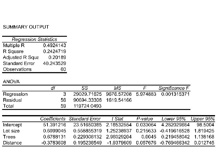
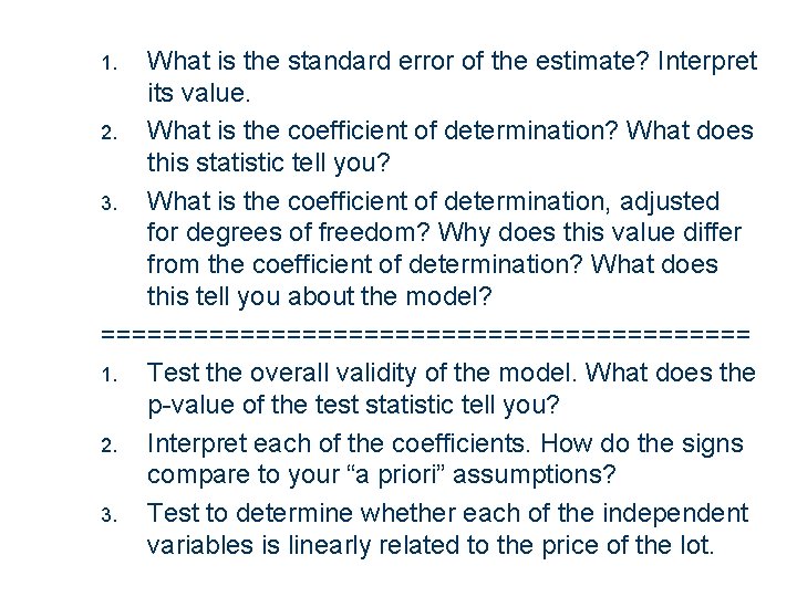
What is the standard error of the estimate? Interpret its value. 2. What is the coefficient of determination? What does this statistic tell you? 3. What is the coefficient of determination, adjusted for degrees of freedom? Why does this value differ from the coefficient of determination? What does this tell you about the model? ===================== 1. Test the overall validity of the model. What does the p-value of the test statistic tell you? 2. Interpret each of the coefficients. How do the signs compare to your “a priori” assumptions? 3. Test to determine whether each of the independent variables is linearly related to the price of the lot. 1. 41

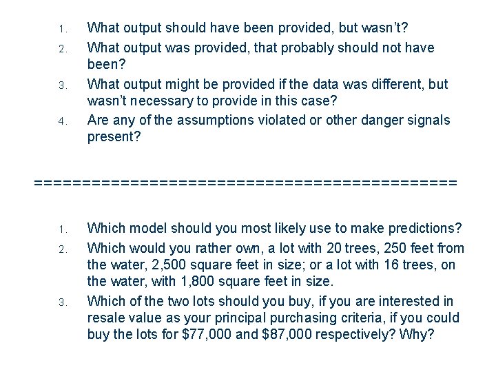
1. 2. 3. 4. What output should have been provided, but wasn’t? What output was provided, that probably should not have been? What output might be provided if the data was different, but wasn’t necessary to provide in this case? Are any of the assumptions violated or other danger signals present? ====================== 1. 2. 3. 42 Which model should you most likely use to make predictions? Which would you rather own, a lot with 20 trees, 250 feet from the water, 2, 500 square feet in size; or a lot with 16 trees, on the water, with 1, 800 square feet in size. Which of the two lots should you buy, if you are interested in resale value as your principal purchasing criteria, if you could buy the lots for $77, 000 and $87, 000 respectively? Why?