Fundamentals of Networking Lab 1 Integrated Sensing Database
Fundamentals of Networking Lab 1 Integrated Sensing & Database Architecture for White Space Networking Sumit Roy Dept. of Electrical Eng. U. Washington, Seattle roy@ee. washington. edu www. ee. washington. edu/research/funlab
2 UW SPECTRUM OBSERVATORY INSIGHTS FROM BUILDING AN OPEN SOURCE SPECTRUM DATABASE FOR TV WHITE SPACE http: //specobs. ee. washington. edu
Fundamentals of Networking Lab 3 Main Take-aways • Databases are based on (predictive) propagation models - these are imperfect at best, and at worst – significantly inaccurate (urban canyons and indoors, in particular) v For TVWS, the FCC mandated the use of F-curves for primary protection, already we can do better (use Longley-Rice) ! § Current Databases leave a lot to be desired in terms of lack of useful supporting analytics; secondary interference modeling is missing (FCC rules only focused on primary protection!) Ø Hence purely using Databases (as per present FCC) to estimate availability of White Spaces is inadvisable need to involve local spectrum measurements to complement Databases!
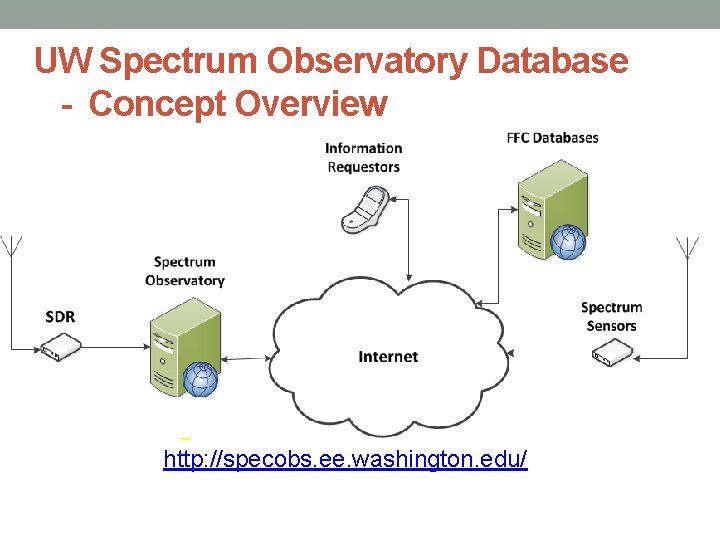
UW Spectrum Observatory Database - Concept Overview http: //specobs. ee. washington. edu/
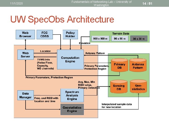
11/1/2020 Fundamentals of Networking Lab – University of Washington UW Spec. Obs Architecture 14 / 51
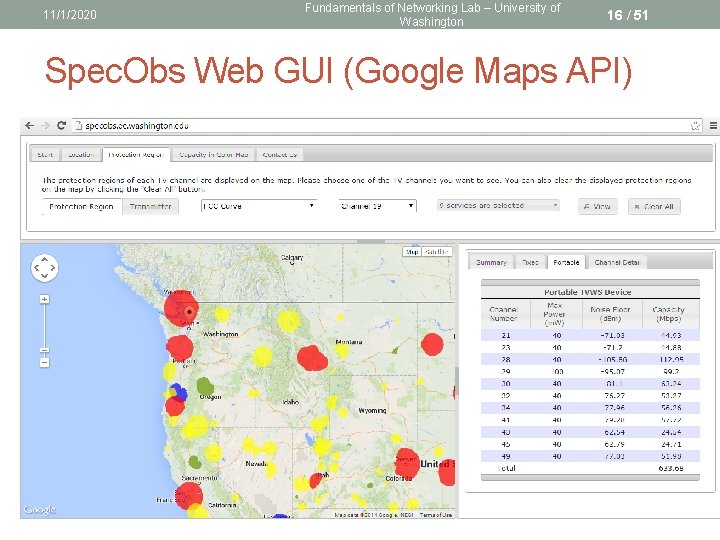
11/1/2020 Fundamentals of Networking Lab – University of Washington 16 / 51 Spec. Obs Web GUI (Google Maps API)
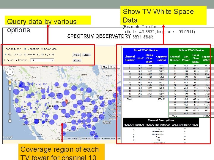
Query data by various options Coverage region of each Show TV White Space Data (Example Data for latitude : 40. 3832, longitude : -96. 0511)
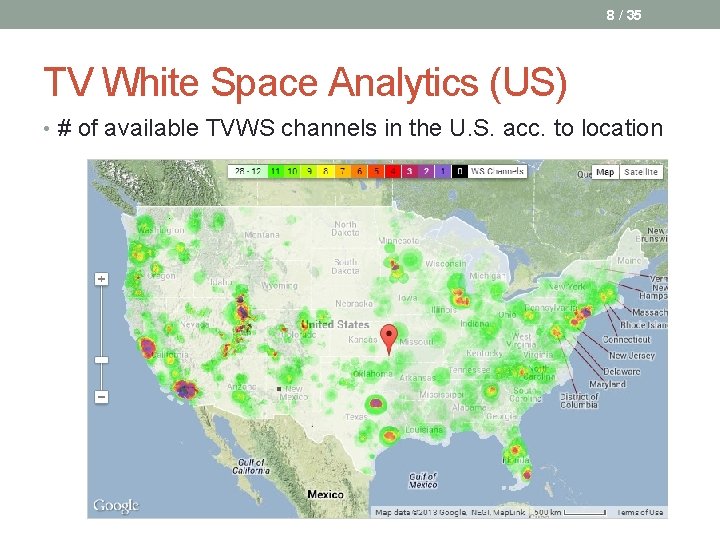
8 / 35 TV White Space Analytics (US) • # of available TVWS channels in the U. S. acc. to location
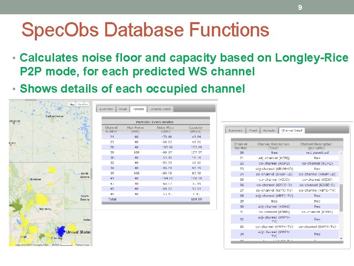
9 Spec. Obs Database Functions • Calculates noise floor and capacity based on Longley-Rice P 2 P mode, for each predicted WS channel • Shows details of each occupied channel
10 FCC - OET Bulletin 69 • Developed in 1990 s for the transition from analog to digital • Determining coverage area and interference using two propagation models - FCC F-Curves and Longley-Rice model • Coverage area • Calculates TV service contours by using F-Curves • Evaluation of TV service • Predicts field strength at the receiver location with Longley-Rice model • Analyzes interference based on predicted field strength “Longley-Rice Methodology for Evaluating TV Coverage and Interference”
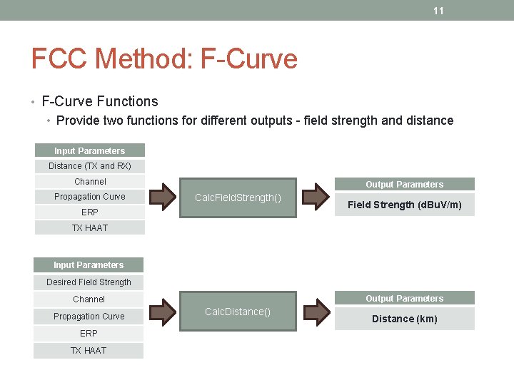
11 FCC Method: F-Curve • F-Curve Functions • Provide two functions for different outputs - field strength and distance Input Parameters Distance (TX and RX) Channel Propagation Curve Output Parameters Calc. Field. Strength() ERP Field Strength (d. Bu. V/m) TX HAAT Input Parameters Desired Field Strength Output Parameters Channel Propagation Curve ERP TX HAAT Calc. Distance() Distance (km)
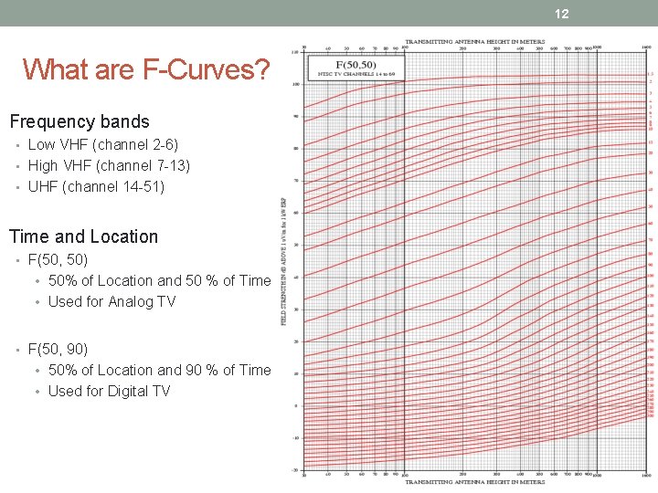
12 What are F-Curves? • Frequency bands • Low VHF (channel 2 -6) • High VHF (channel 7 -13) • UHF (channel 14 -51) • Time and Location • F(50, 50) • 50% of Location and 50 % of Time • Used for Analog TV • F(50, 90) • 50% of Location and 90 % of Time • Used for Digital TV
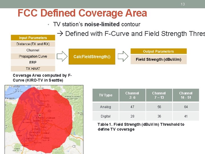
13 FCC Defined Coverage Area • TV station’s noise-limited contour Defined with F-Curve and Field Strength Thres Coverage Area computed by FCurve (KIRO-TV in Seattle) TV Type Channel 2 - 6 Channel 7 – 13 Channel 14 - 51 Analog 47 56 64 Digital 28 36 41 Table 1. Field Strength (d. Bu. V/m) Threshold to define TV coverage
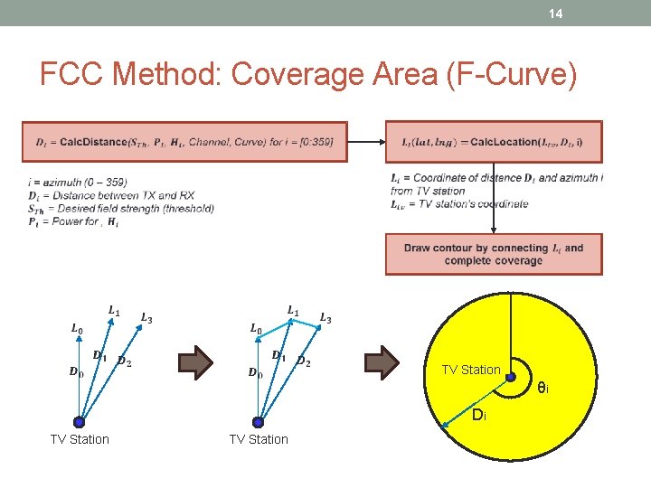
14 FCC Method: Coverage Area (F-Curve) TV Station θi Di TV Station
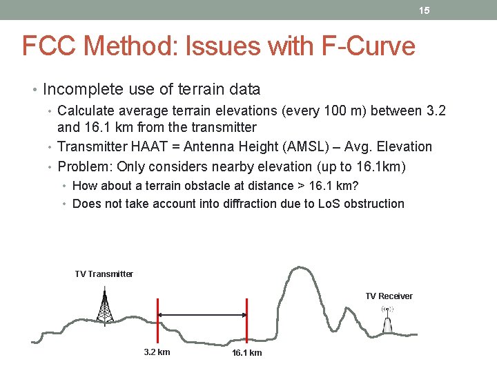
15 FCC Method: Issues with F-Curve • Incomplete use of terrain data • Calculate average terrain elevations (every 100 m) between 3. 2 and 16. 1 km from the transmitter • Transmitter HAAT = Antenna Height (AMSL) – Avg. Elevation • Problem: Only considers nearby elevation (up to 16. 1 km) • How about a terrain obstacle at distance > 16. 1 km? • Does not take account into diffraction due to Lo. S obstruction TV Transmitter TV Receiver 3. 2 km 16. 1 km
Longley-Rice model for Path LOSS PREDICTION IRREGULAR TERRAIN MODEL • Statistical/semi-empirical model - includes terrain specific inputs - Empirically weights loss components from knife edge diffraction with those from multipath propagation • Adopted as a standard by the NTIA v Wide range of applicability: 20 MHz- 40 GHz; upto 2000 Km low & high altitude scenarios • Many software implementations available commercially • Includes most relevant propagation modes v multiple knife & rounded edge diffraction (irregular terrain), atmospheric attenuation, tropospheric propagation
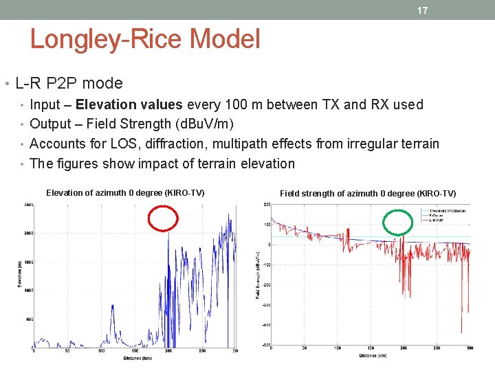
17 Longley-Rice Model • L-R P 2 P mode • Input – Elevation values every 100 m between TX and RX used • Output – Field Strength (d. Bu. V/m) • Accounts for LOS, diffraction, multipath effects from irregular terrain • The figures show impact of terrain elevation Elevation of azimuth 0 degree (KIRO-TV) Field strength of azimuth 0 degree (KIRO-TV)
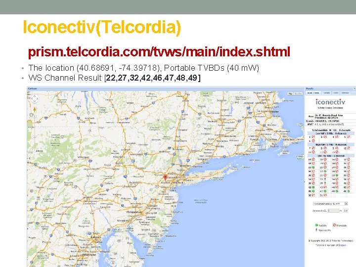
Iconectiv(Telcordia) prism. telcordia. com/tvws/main/index. shtml • The location (40. 68691, -74. 39718), Portable TVBDs (40 m. W) • WS Channel Result [22, 27, 32, 46, 47, 48, 49]
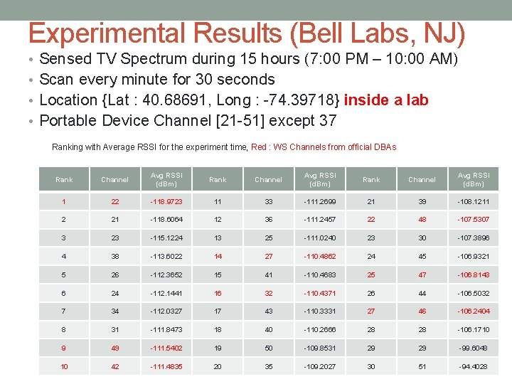
Experimental Results (Bell Labs, NJ) • Sensed TV Spectrum during 15 hours (7: 00 PM – 10: 00 AM) • Scan every minute for 30 seconds • Location {Lat : 40. 68691, Long : -74. 39718} inside a lab • Portable Device Channel [21 -51] except 37 Ranking with Average RSSI for the experiment time, Red : WS Channels from official DBAs Rank Channel Avg RSSI (d. Bm) 1 22 -118. 9723 11 33 -111. 2699 21 39 -108. 1211 2 21 -118. 6064 12 36 -111. 2457 22 48 -107. 5307 3 23 -115. 1224 13 25 -111. 0240 23 30 -107. 3896 4 38 -113. 6022 14 27 -110. 4862 24 45 -106. 9321 5 26 -112. 3652 15 41 -110. 4683 25 47 -106. 8143 6 24 -112. 1441 16 32 -110. 4371 26 44 -106. 5032 7 34 -112. 0327 17 43 -110. 3331 27 46 -106. 2404 8 31 -111. 8473 18 40 -110. 2666 28 28 -106. 1710 9 49 -111. 5402 19 50 -109. 8531 29 29 -99. 6048 10 42 -111. 4835 20 35 -109. 2027 30 51 -94. 4028
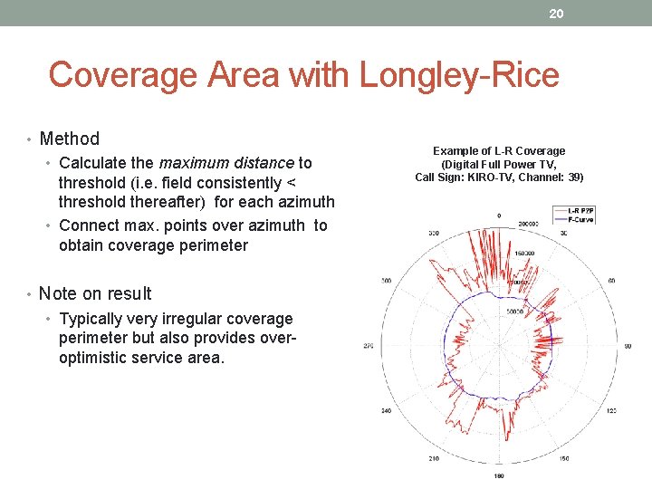
20 Coverage Area with Longley-Rice • Method • Calculate the maximum distance to threshold (i. e. field consistently < threshold thereafter) for each azimuth • Connect max. points over azimuth to obtain coverage perimeter • Note on result • Typically very irregular coverage perimeter but also provides overoptimistic service area. Example of L-R Coverage (Digital Full Power TV, Call Sign: KIRO-TV, Channel: 39)
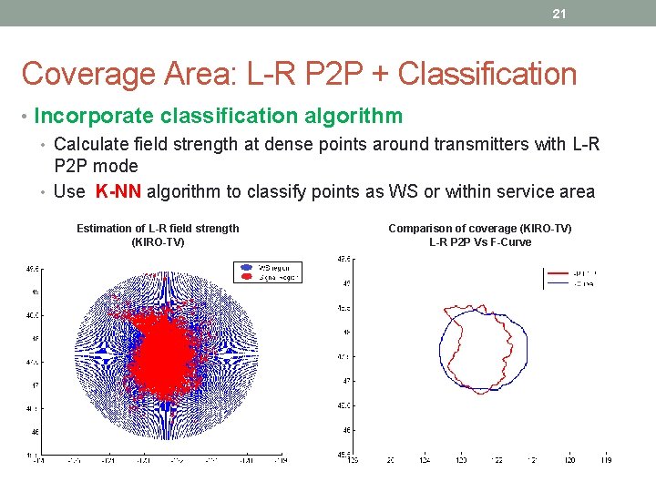
21 Coverage Area: L-R P 2 P + Classification • Incorporate classification algorithm • Calculate field strength at dense points around transmitters with L-R P 2 P mode • Use K-NN algorithm to classify points as WS or within service area Estimation of L-R field strength (KIRO-TV) Comparison of coverage (KIRO-TV) L-R P 2 P Vs F-Curve
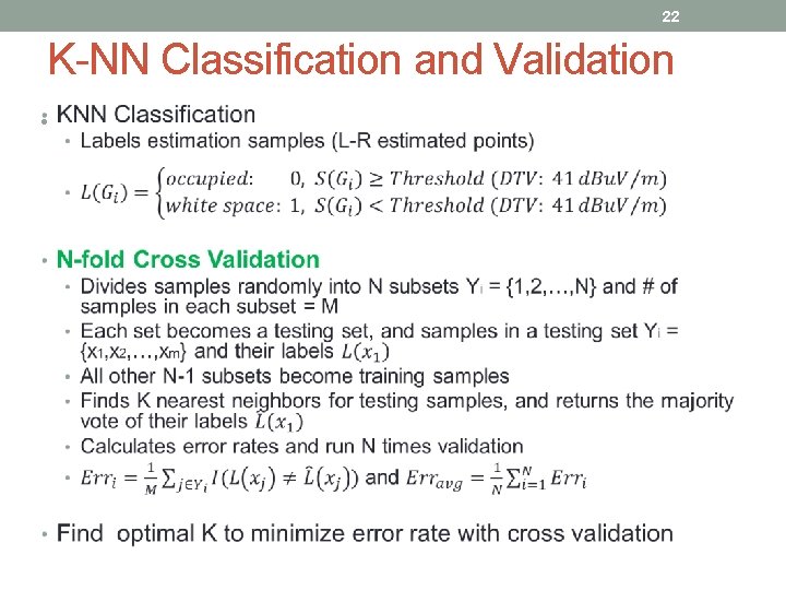
22 K-NN Classification and Validation •
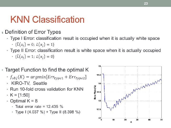
23 KNN Classification •
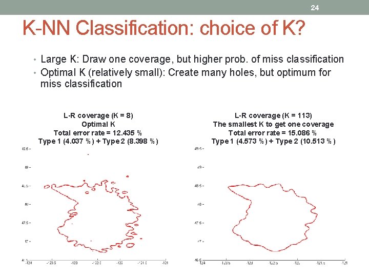
24 K-NN Classification: choice of K? • Large K: Draw one coverage, but higher prob. of miss classification • Optimal K (relatively small): Create many holes, but optimum for miss classification L-R coverage (K = 8) Optimal K Total error rate = 12. 435 % Type 1 (4. 037 %) + Type 2 (8. 398 %) L-R coverage (K = 113) The smallest K to get one coverage Total error rate = 15. 086 % Type 1 (4. 573 %) + Type 2 (10. 513 %)
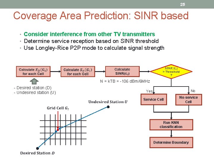
25 Coverage Area Prediction: SINR based • Consider interference from other TV transmitters • Determine service reception based on SINR threshold • Use Longley-Rice P 2 P mode to calculate signal strength N = k. TB = -106 d. Bm/6 MHz - Desired station (D) - Undesired station (U) No Yes Service Cell No-service Cell Run KNN classification Determine Boundary
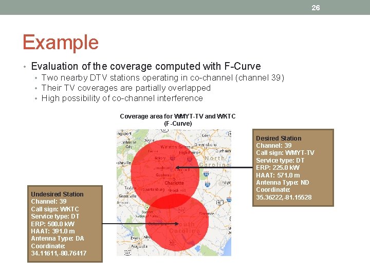
26 Example • Evaluation of the coverage computed with F-Curve • Two nearby DTV stations operating in co-channel (channel 39) • Their TV coverages are partially overlapped • High possibility of co-channel interference Coverage area for WMYT-TV and WKTC (F-Curve) Undesired Station Channel: 39 Call sign: WKTC Service type: DT ERP: 500. 0 k. W HAAT: 391. 0 m Antenna Type: DA Coordinate: 34. 11611, -80. 76417 Desired Station Channel: 39 Call sign: WMYT-TV Service type: DT ERP: 225. 0 k. W HAAT: 571. 0 m Antenna Type: ND Coordinate: 35. 36222, -81. 15528
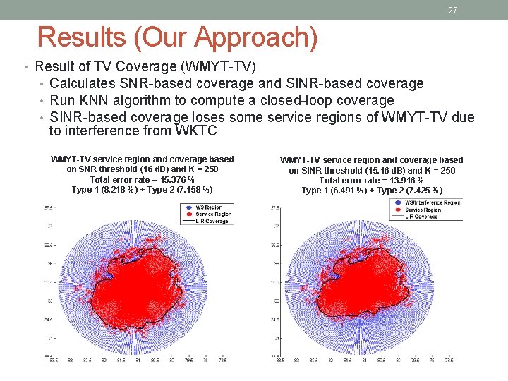
27 Results (Our Approach) • Result of TV Coverage (WMYT-TV) • Calculates SNR-based coverage and SINR-based coverage • Run KNN algorithm to compute a closed-loop coverage • SINR-based coverage loses some service regions of WMYT-TV due to interference from WKTC WMYT-TV service region and coverage based on SNR threshold (16 d. B) and K = 250 Total error rate = 15. 376 % Type 1 (8. 218 %) + Type 2 (7. 158 %) WMYT-TV service region and coverage based on SINR threshold (15. 16 d. B) and K = 250 Total error rate = 13. 916 % Type 1 (6. 491 %) + Type 2 (7. 425 %)
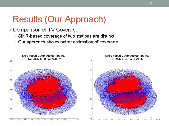
28 Results (Our Approach) • Comparison of TV Coverage • SINR-based coverage of two stations are distinct • Our approach shows better estimation of coverage SNR-based Coverage comparison for WMYT-TV and WKTC SINR-based Coverage comparison for WMYT-TV and WKTC
Fundamentals of Networking Lab 29 Towards Data-driven White Space Maps q State of Spectrum Measurements very spotty - data not publicly available - no continuous monitoring - point data, almost no driving data (i. e. area coverage) need robust vehicle-friendly platforms and commitment to sustained open source data campaigns !
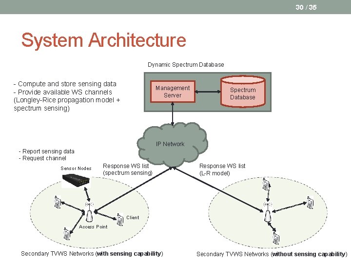
30 / 35 System Architecture Dynamic Spectrum Database - Compute and store sensing data - Provide available WS channels (Longley-Rice propagation model + spectrum sensing) Management Server Spectrum Database IP Network - Report sensing data - Request channel Sensor Nodes Response WS list (spectrum sensing) Response WS list (L-R model) Client Access Point Secondary TVWS Networks (with sensing capability) Secondary TVWS Networks (without sensing capability)
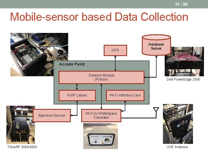
31 / 35 Mobile-sensor based Data Collection GPS Database Server Access Point Daemon Module (Python) Py. RF Library Spectrum Sensor Think. RF WSA 4000 Dell Power. Edge 2950 Wi-Fi Interface Card Wi-Fi to White. Space Translator UHF Antenna
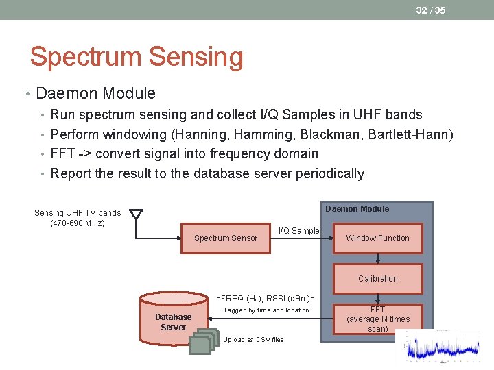
32 / 35 Spectrum Sensing • Daemon Module • Run spectrum sensing and collect I/Q Samples in UHF bands • Perform windowing (Hanning, Hamming, Blackman, Bartlett-Hann) • FFT -> convert signal into frequency domain • Report the result to the database server periodically Daemon Module Sensing UHF TV bands (470 -698 MHz) Spectrum Sensor I/Q Sample Window Function Calibration <FREQ (Hz), RSSI (d. Bm)> Database Server Tagged by time and location Upload as CSV files FFT (average N times scan)
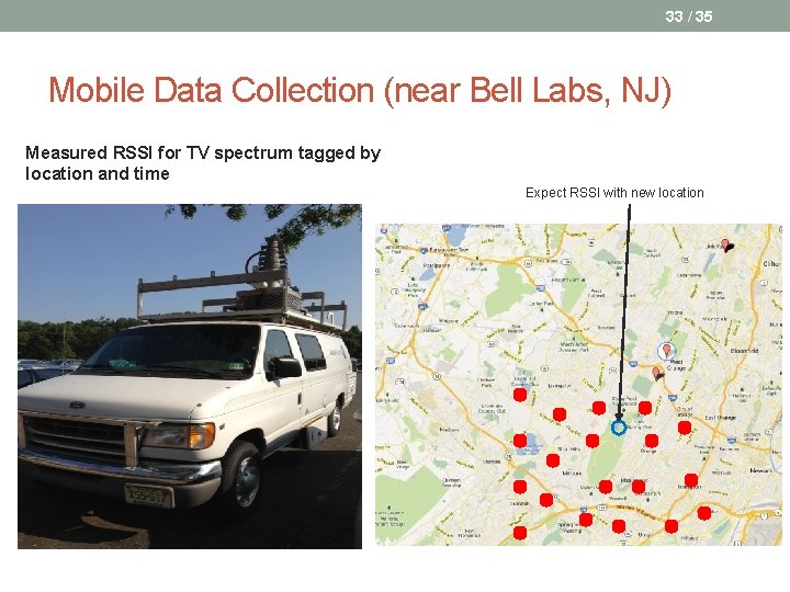
33 / 35 Mobile Data Collection (near Bell Labs, NJ) Measured RSSI for TV spectrum tagged by location and time Expect RSSI with new location
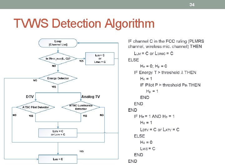
34 TVWS Detection Algorithm DTV Analog TV
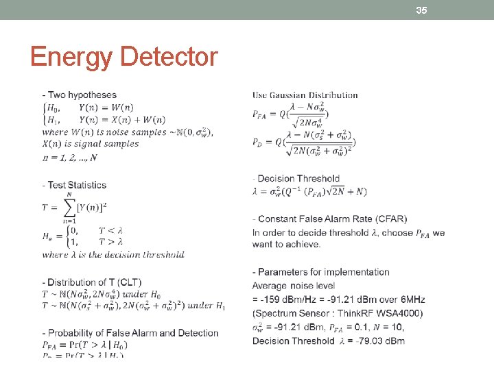
35 Energy Detector
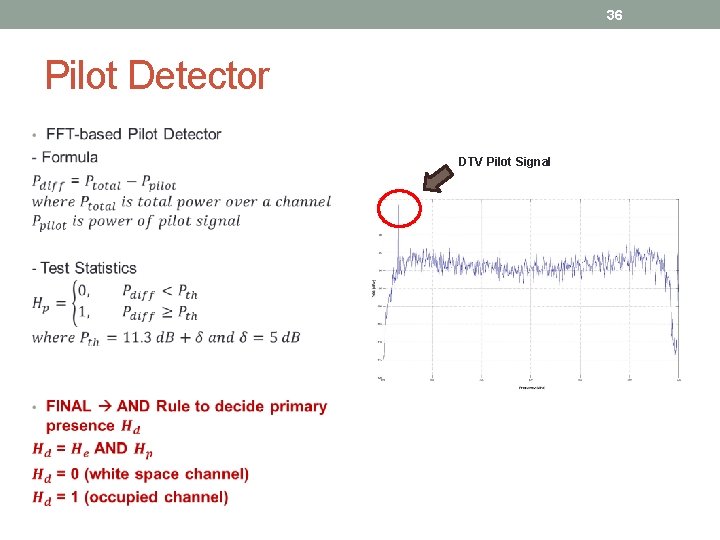
36 Pilot Detector DTV Pilot Signal
![37 / 35 Primary Detection Algorithm Loop [Channel List] Energy & Pilot Detection Pg 37 / 35 Primary Detection Algorithm Loop [Channel List] Energy & Pilot Detection Pg](http://slidetodoc.com/presentation_image/3963c7e1a0948736319c612bb1a4bc77/image-37.jpg)
37 / 35 Primary Detection Algorithm Loop [Channel List] Energy & Pilot Detection Pg = Logical AND Pg = 0? Mark as white space channel FCC rules Delete from white space channel Last Channel? Terminate
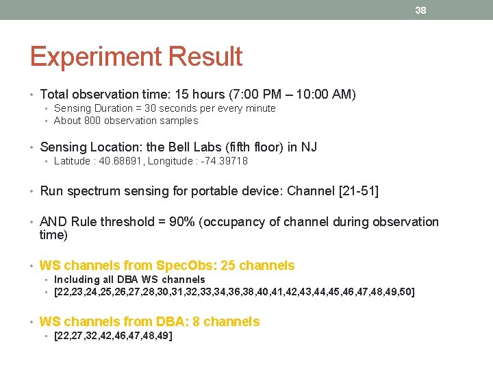
38 Experiment Result • Total observation time: 15 hours (7: 00 PM – 10: 00 AM) • Sensing Duration = 30 seconds per every minute • About 800 observation samples • Sensing Location: the Bell Labs (fifth floor) in NJ • Latitude : 40. 68691, Longitude : -74. 39718 • Run spectrum sensing for portable device: Channel [21 -51] • AND Rule threshold = 90% (occupancy of channel during observation time) • WS channels from Spec. Obs: 25 channels • Including all DBA WS channels • [22, 23, 24, 25, 26, 27, 28, 30, 31, 32, 33, 34, 36, 38, 40, 41, 42, 43, 44, 45, 46, 47, 48, 49, 50] • WS channels from DBA: 8 channels • [22, 27, 32, 46, 47, 48, 49]
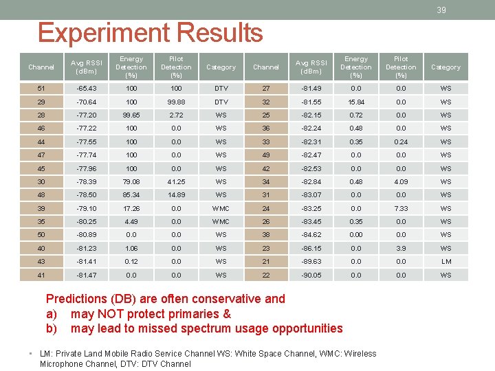
39 Experiment Results Channel Avg RSSI (d. Bm) Energy Detection (%) Pilot Detection (%) Category 51 -65. 43 100 DTV 27 -81. 49 0. 0 WS 29 -70. 64 100 99. 88 DTV 32 -81. 55 15. 84 0. 0 WS 28 -77. 20 99. 65 2. 72 WS 25 -82. 15 0. 72 0. 0 WS 46 -77. 22 100 0. 0 WS 36 -82. 24 0. 48 0. 0 WS 44 -77. 55 100 0. 0 WS 33 -82. 31 0. 35 0. 24 WS 47 -77. 74 100 0. 0 WS 49 -82. 47 0. 0 WS 45 -77. 96 100 0. 0 WS 42 -82. 53 0. 0 WS 30 -78. 39 79. 08 41. 25 WS 34 -82. 84 0. 48 4. 09 WS 48 -78. 50 85. 34 14. 89 WS 31 -83. 07 0. 0 WS 39 -79. 10 17. 26 0. 0 WMC 24 -83. 25 0. 0 7. 33 WS 35 -80. 25 4. 49 0. 0 WMC 26 -83. 45 0. 35 0. 0 WS 50 -80. 89 0. 0 WS 38 -84. 62 0. 00 0. 0 WS 40 -81. 23 1. 06 0. 0 WS 23 -86. 15 0. 0 3. 9 WS 43 -81. 41 0. 12 0. 0 WS 21 -89. 63 0. 0 LM 41 -81. 47 0. 0 WS 22 -90. 05 0. 0 WS Predictions (DB) are often conservative and a) may NOT protect primaries & b) may lead to missed spectrum usage opportunities • LM: Private Land Mobile Radio Service Channel WS: White Space Channel, WMC: Wireless Microphone Channel, DTV: DTV Channel
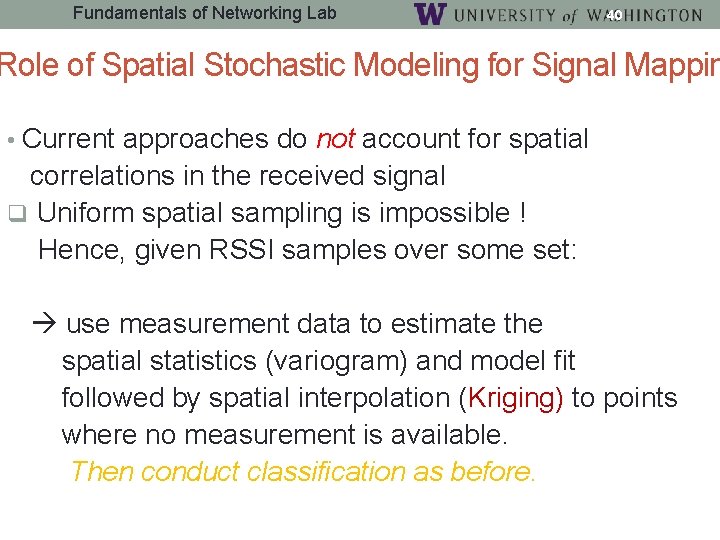
Fundamentals of Networking Lab 40 Role of Spatial Stochastic Modeling for Signal Mappin • Current approaches do not account for spatial correlations in the received signal q Uniform spatial sampling is impossible ! Hence, given RSSI samples over some set: use measurement data to estimate the spatial statistics (variogram) and model fit followed by spatial interpolation (Kriging) to points where no measurement is available. Then conduct classification as before.
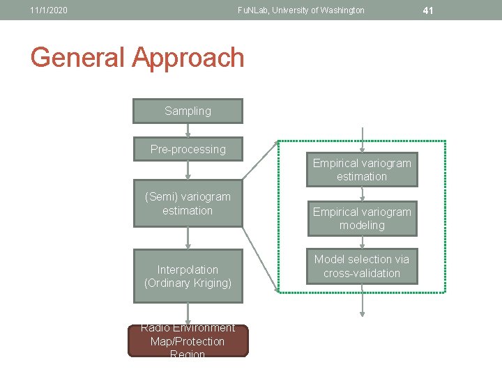
11/1/2020 Fu. NLab, University of Washington General Approach Sampling Pre-processing Empirical variogram estimation (Semi) variogram estimation Interpolation (Ordinary Kriging) Radio Environment Map/Protection Region Empirical variogram modeling Model selection via cross-validation 41
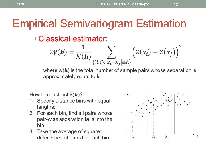
11/1/2020 Fu. NLab, University of Washington 42 Empirical Semivariogram Estimation •
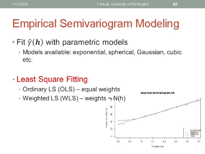
11/1/2020 Fu. NLab, University of Washington 43 Empirical Semivariogram Modeling •
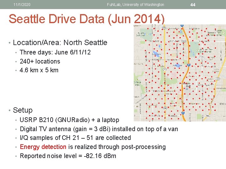
11/1/2020 Fu. NLab, University of Washington Seattle Drive Data (Jun 2014) • Location/Area: North Seattle • Three days: June 6/11/12 • 240+ locations • 4. 6 km x 5 km • Setup • USRP B 210 (GNURadio) + a laptop • Digital TV antenna (gain = 3 d. Bi) installed on top of a van • I/Q samples of CH 21 – 51 are collected • Energy detection is realized through post-processing • Reported noise level = -82. 16 d. Bm 44
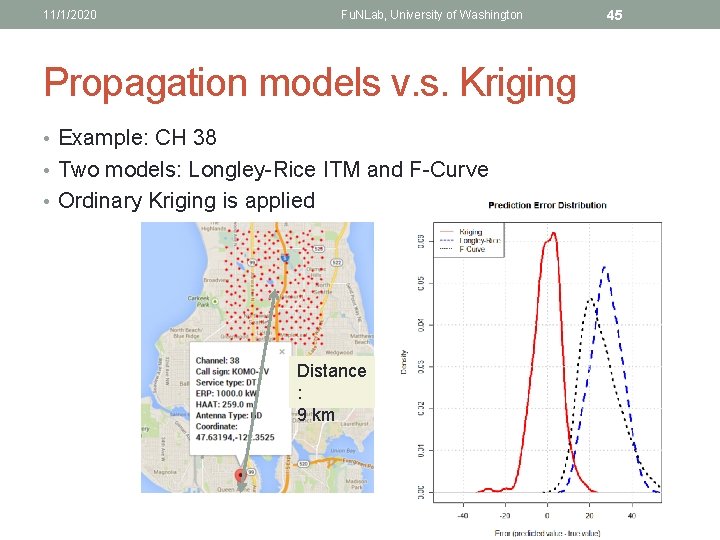
11/1/2020 Fu. NLab, University of Washington Propagation models v. s. Kriging • Example: CH 38 • Two models: Longley-Rice ITM and F-Curve • Ordinary Kriging is applied Distance : 9 km 45
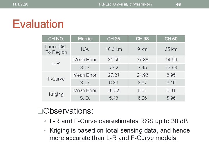
11/1/2020 46 Fu. NLab, University of Washington Evaluation CH NO. Metric CH 25 CH 38 CH 50 Tower Dist. To Region N/A 10. 6 km 9 km 35 km Mean Error 31. 59 27. 86 14. 99 S. D. 7. 42 7. 45 12. 93 Mean Error 27. 27 24. 93 8. 95 S. D. 6. 80 8. 97 9. 10 Mean Error -0. 02 0. 01 S. D. 5. 48 6. 26 5. 96 L-R F-Curve Kriging �Observations: ◦ L-R and F-Curve overestimates RSS up to 30 d. B. ◦ Kriging is based on local sensing data, and hence more accurate than L-R and F-Curve models.
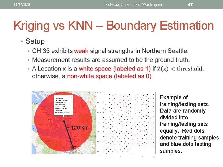
11/1/2020 Fu. NLab, University of Washington 47 Kriging vs KNN – Boundary Estimation • ~120 km Example of training/testing sets. Data are randomly divided into training/testing sets equally. Red dots denote training samples, and blue dots testing samples.
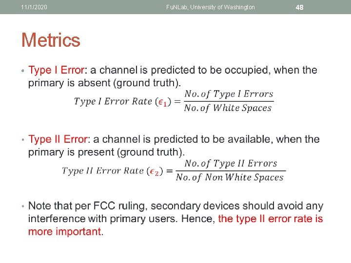
11/1/2020 Metrics • Fu. NLab, University of Washington 48
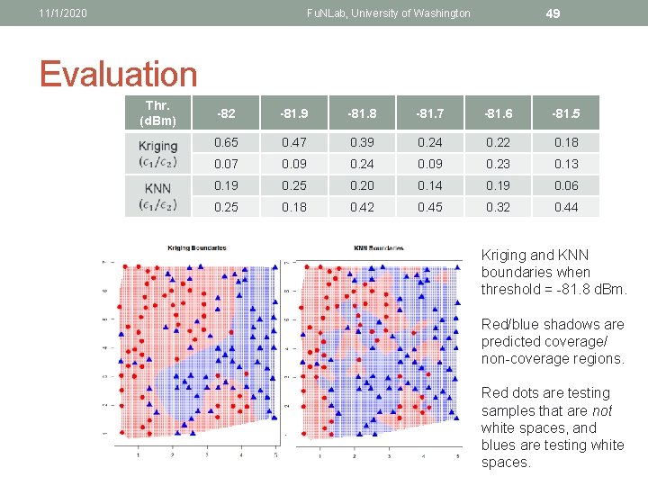
11/1/2020 49 Fu. NLab, University of Washington Evaluation Thr. (d. Bm) -82 -81. 9 -81. 8 -81. 7 -81. 6 -81. 5 0. 65 0. 47 0. 39 0. 24 0. 22 0. 18 0. 07 0. 09 0. 24 0. 09 0. 23 0. 19 0. 25 0. 20 0. 14 0. 19 0. 06 0. 25 0. 18 0. 42 0. 45 0. 32 0. 44 Kriging and KNN boundaries when threshold = -81. 8 d. Bm. Red/blue shadows are predicted coverage/ non-coverage regions. Red dots are testing samples that are not white spaces, and blues are testing white spaces.
Fundamentals of Networking Lab 50 Conclusions • Work in Progress just the beginning in Large Scale Radio Mapping!
- Slides: 50