Fundamentals of Fluid Mechanics Chapter 7 DIMENSIONAL ANALYSIS

Fundamentals of Fluid Mechanics Chapter 7: DIMENSIONAL ANALYSIS AND MODELING Department of Hydraulic Engineering School of Civil Engineering Shandong University 2007

Objectives Understand dimensions, units, and dimensional homogeneity Understand benefits of dimensional analysis Know how to use the method of repeating variables Understand the concept of similarity and how to apply it to experimental modeling Fundamentals of Fluid Mechanics 2 Chapter 7: DIMENSIONAL ANALYSIS AND MODELING

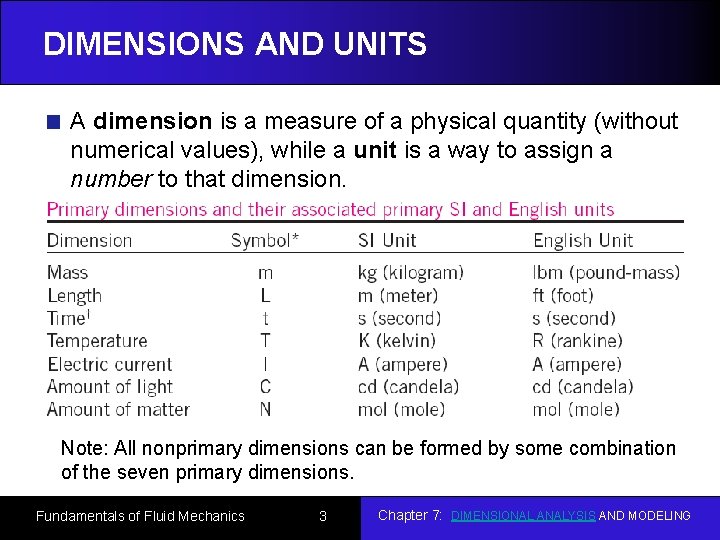
DIMENSIONS AND UNITS A dimension is a measure of a physical quantity (without numerical values), while a unit is a way to assign a number to that dimension. Note: All nonprimary dimensions can be formed by some combination of the seven primary dimensions. Fundamentals of Fluid Mechanics 3 Chapter 7: DIMENSIONAL ANALYSIS AND MODELING

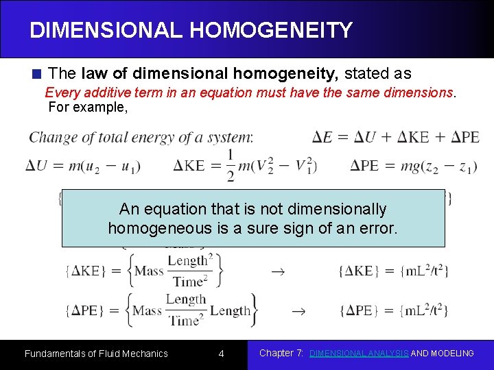
DIMENSIONAL HOMOGENEITY The law of dimensional homogeneity, stated as Every additive term in an equation must have the same dimensions. For example, An equation that is not dimensionally homogeneous is a sure sign of an error. Fundamentals of Fluid Mechanics 4 Chapter 7: DIMENSIONAL ANALYSIS AND MODELING

Nondimensionalization of Equations Dimensional homogeneity every term in an equation has the same dimensions. nondimensional divide each term in the equation by a collection of variables and constants whose product has those same dimensions. If the nondimensional terms in the equation are of order unity called normalized. Normalization is thus more restrictive than nondimensionalization. (often used interchangeably). Nondimensional parameters are named after a notable scientist or engineer (e. g. , the Reynolds number and the Froude number). This process is referred to by some authors as inspectional analysis. Fundamentals of Fluid Mechanics 5 Chapter 7: DIMENSIONAL ANALYSIS AND MODELING

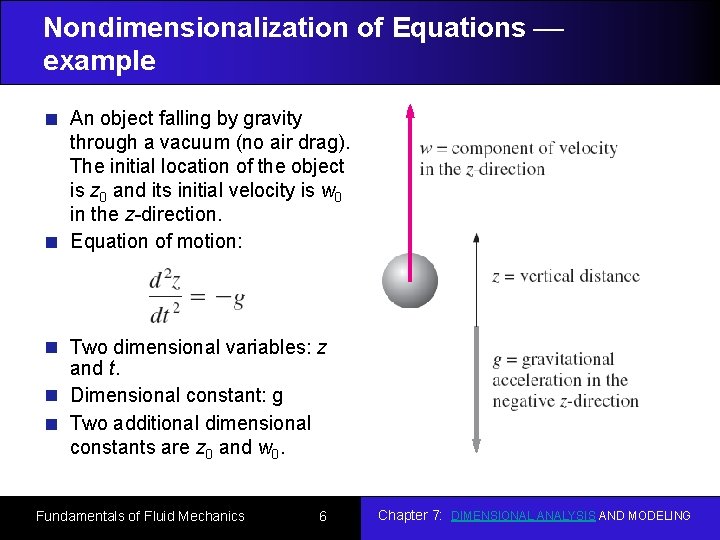
Nondimensionalization of Equations example An object falling by gravity through a vacuum (no air drag). The initial location of the object is z 0 and its initial velocity is w 0 in the z-direction. Equation of motion: Two dimensional variables: z and t. Dimensional constant: g Two additional dimensional constants are z 0 and w 0. Fundamentals of Fluid Mechanics 6 Chapter 7: DIMENSIONAL ANALYSIS AND MODELING

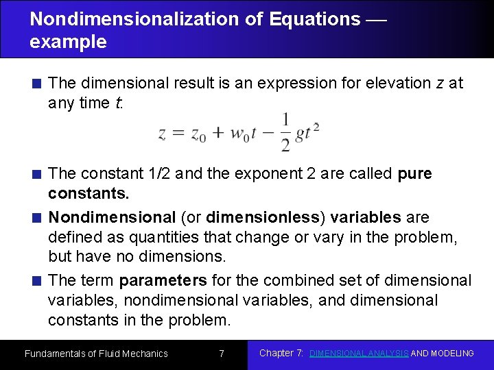
Nondimensionalization of Equations example The dimensional result is an expression for elevation z at any time t: The constant 1/2 and the exponent 2 are called pure constants. Nondimensional (or dimensionless) variables are defined as quantities that change or vary in the problem, but have no dimensions. The term parameters for the combined set of dimensional variables, nondimensional variables, and dimensional constants in the problem. Fundamentals of Fluid Mechanics 7 Chapter 7: DIMENSIONAL ANALYSIS AND MODELING

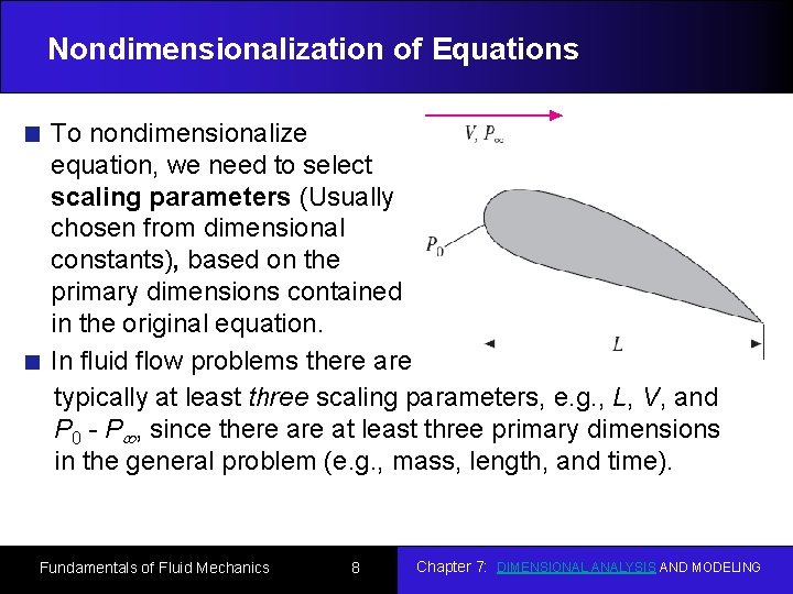
Nondimensionalization of Equations To nondimensionalize equation, we need to select scaling parameters (Usually chosen from dimensional constants), based on the primary dimensions contained in the original equation. In fluid flow problems there are typically at least three scaling parameters, e. g. , L, V, and P 0 - P , since there at least three primary dimensions in the general problem (e. g. , mass, length, and time). Fundamentals of Fluid Mechanics 8 Chapter 7: DIMENSIONAL ANALYSIS AND MODELING

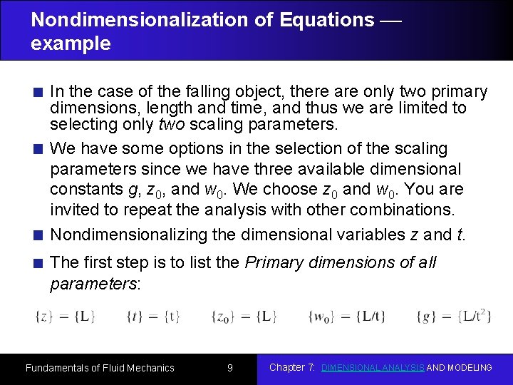
Nondimensionalization of Equations example In the case of the falling object, there are only two primary dimensions, length and time, and thus we are limited to selecting only two scaling parameters. We have some options in the selection of the scaling parameters since we have three available dimensional constants g, z 0, and w 0. We choose z 0 and w 0. You are invited to repeat the analysis with other combinations. Nondimensionalizing the dimensional variables z and t. The first step is to list the Primary dimensions of all parameters: Fundamentals of Fluid Mechanics 9 Chapter 7: DIMENSIONAL ANALYSIS AND MODELING

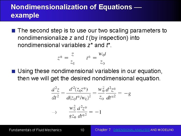
Nondimensionalization of Equations example The second step is to use our two scaling parameters to nondimensionalize z and t (by inspection) into nondimensional variables z* and t*. Using these nondimensional variables in our equation, then we will get the desired nondimensional equation. Fundamentals of Fluid Mechanics 10 Chapter 7: DIMENSIONAL ANALYSIS AND MODELING

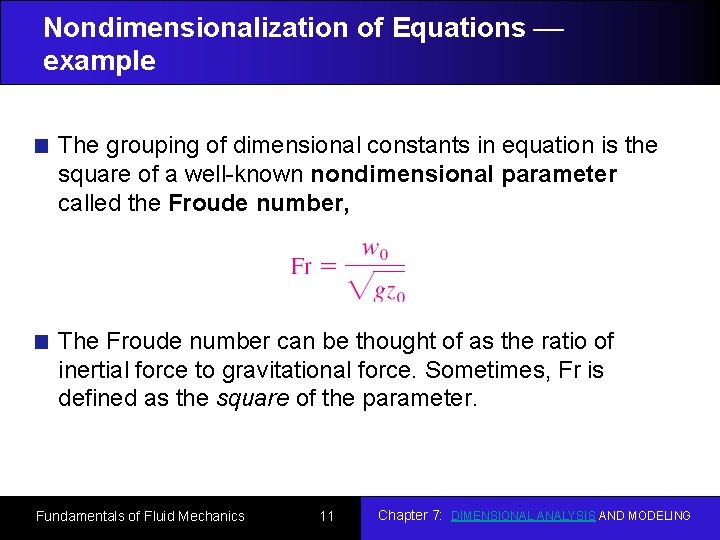
Nondimensionalization of Equations example The grouping of dimensional constants in equation is the square of a well-known nondimensional parameter called the Froude number, The Froude number can be thought of as the ratio of inertial force to gravitational force. Sometimes, Fr is defined as the square of the parameter. Fundamentals of Fluid Mechanics 11 Chapter 7: DIMENSIONAL ANALYSIS AND MODELING

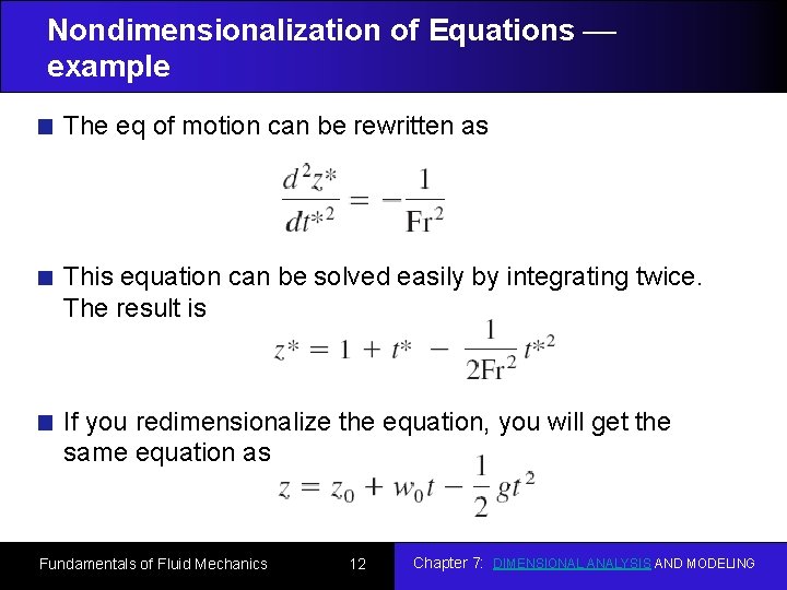
Nondimensionalization of Equations example The eq of motion can be rewritten as This equation can be solved easily by integrating twice. The result is If you redimensionalize the equation, you will get the same equation as Fundamentals of Fluid Mechanics 12 Chapter 7: DIMENSIONAL ANALYSIS AND MODELING

Nondimensionalization of Equations example What then is the advantage of nondimensionalizing the equation? There are two key advantages of nondimensionalization. First, it increases our insight about the relationships between key parameters. for example, that doubling w 0 has the same effect as decreasing z 0 by a factor of 4. Second, it reduces the number of parameters in the problem. For example, original problem contains one z; one t; and three additional dimensional constants, g, w 0, and z 0. The nondimensionalized problem contains one z*; one t*; and only one additional parameter, Fr. Fundamentals of Fluid Mechanics 13 Chapter 7: DIMENSIONAL ANALYSIS AND MODELING

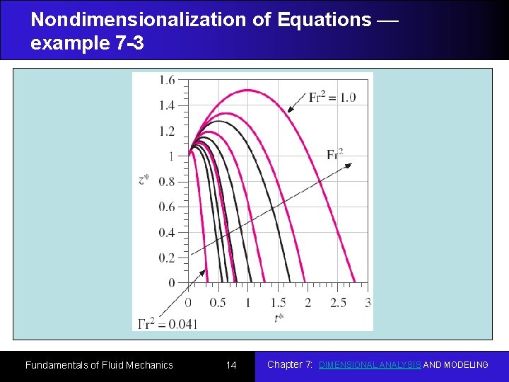
Nondimensionalization of Equations example 7 -3 An object falling by gravity through a vacuum (no air drag) in a vertical pipe. The initial location of the object is z 0 and its initial velocity is w 0 in the z-direction. Fundamentals of Fluid Mechanics 14 Chapter 7: DIMENSIONAL ANALYSIS AND MODELING

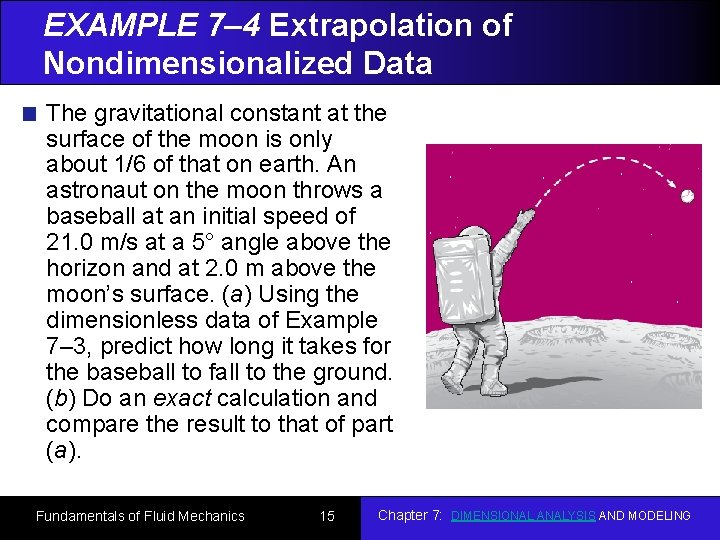
EXAMPLE 7– 4 Extrapolation of Nondimensionalized Data The gravitational constant at the surface of the moon is only about 1/6 of that on earth. An astronaut on the moon throws a baseball at an initial speed of 21. 0 m/s at a 5° angle above the horizon and at 2. 0 m above the moon’s surface. (a) Using the dimensionless data of Example 7– 3, predict how long it takes for the baseball to fall to the ground. (b) Do an exact calculation and compare the result to that of part (a). Fundamentals of Fluid Mechanics 15 Chapter 7: DIMENSIONAL ANALYSIS AND MODELING

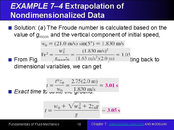
EXAMPLE 7– 4 Extrapolation of Nondimensionalized Data Solution: (a) The Froude number is calculated based on the value of gmoon and the vertical component of initial speed, From Fig. 7 -13, we can find t* = 2. 75, Converting back to dimensional variables, we can get Exact time to strike the ground: Fundamentals of Fluid Mechanics 16 Chapter 7: DIMENSIONAL ANALYSIS AND MODELING

DIMENSIONAL ANALYSIS AND SIMILARITY Nondimensionalization of an equation is useful only when the equation is known! In many real-world flows, the equations are either unknown or too difficult to solve. Experimentation is the only method of obtaining reliable information In most experiments, geometrically–scaled models are used (time and money). Experimental conditions and results must be properly scaled so that results are meaningful for the full-scale prototype. Therefore, Dimensional Analysis Fundamentals of Fluid Mechanics 17 Chapter 7: DIMENSIONAL ANALYSIS AND MODELING

DIMENSIONAL ANALYSIS AND SIMILARITY Primary purposes of dimensional analysis To generate nondimensional parameters that help in the design of experiments (physical and/or numerical) and in reporting of results. To obtain scaling laws so that prototype performance can be predicted from model performance. To predict trends in the relationship between parameters. Fundamentals of Fluid Mechanics 18 Chapter 7: DIMENSIONAL ANALYSIS AND MODELING

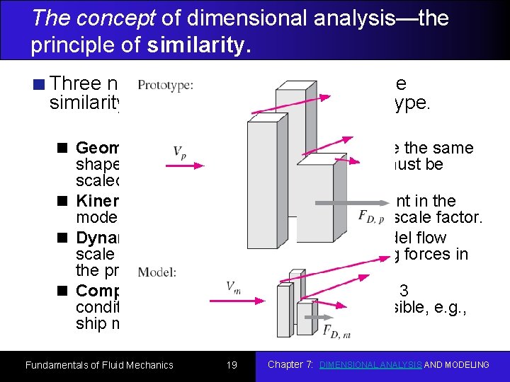
The concept of dimensional analysis—the principle of similarity. Three necessary conditions for complete similarity between a model and a prototype. Geometric Similarity – the model must be the same shape as the prototype. Each dimension must be scaled by the same factor. Kinematic Similarity – velocity as any point in the model must be proportional by a constant scale factor. Dynamic Similarity – all forces in the model flow scale by a constant factor to corresponding forces in the prototype flow. Complete Similarity is achieved only if all 3 conditions are met. This is not always possible, e. g. , ship models. Fundamentals of Fluid Mechanics 19 Chapter 7: DIMENSIONAL ANALYSIS AND MODELING

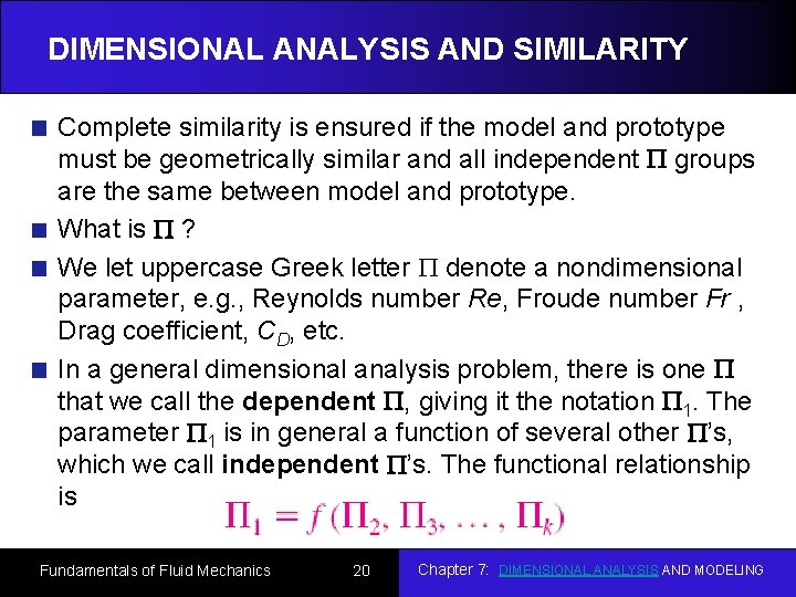
DIMENSIONAL ANALYSIS AND SIMILARITY Complete similarity is ensured if the model and prototype must be geometrically similar and all independent groups are the same between model and prototype. What is ? We let uppercase Greek letter denote a nondimensional parameter, e. g. , Reynolds number Re, Froude number Fr , Drag coefficient, CD, etc. In a general dimensional analysis problem, there is one that we call the dependent , giving it the notation 1. The parameter 1 is in general a function of several other ’s, which we call independent ’s. The functional relationship is Fundamentals of Fluid Mechanics 20 Chapter 7: DIMENSIONAL ANALYSIS AND MODELING

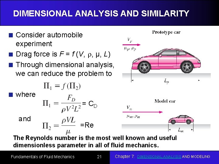
DIMENSIONAL ANALYSIS AND SIMILARITY Consider automobile experiment Drag force is F = f (V, , µ, L) Through dimensional analysis, we can reduce the problem to where = CD and =Re The Reynolds number is the most well known and useful dimensionless parameter in all of fluid mechanics. Fundamentals of Fluid Mechanics 21 Chapter 7: DIMENSIONAL ANALYSIS AND MODELING

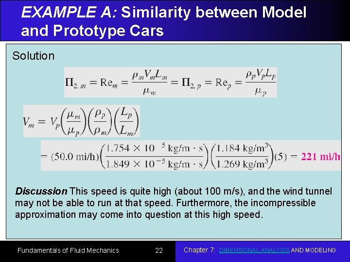
EXAMPLE A: Similarity between Model and Prototype Cars The aerodynamic drag of a new Solution sports car is to be predicted at a speed of 50. 0 mi/h at an air temperature of 25°C. Automotive engineers build a one-fifth scale model of the car to test in a wind tunnel. It is winter and the wind tunnel is located in an unheated building; the temperature of the wind tunnel air is only about 5°C. Determine how fast the Discussion speedrun is quite engineers. This should the high wind(about 100 m/s), and the wind tunnel may not be to run at that speed. Furthermore, the incompressible tunnel inable order to achieve approximation may come intomodel question at this high speed. similarity between the and the prototype. Fundamentals of Fluid Mechanics 22 Chapter 7: DIMENSIONAL ANALYSIS AND MODELING

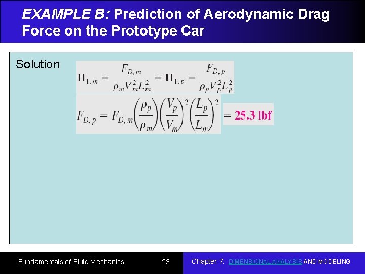
EXAMPLE B: Prediction of Aerodynamic Drag Force on the Prototype Car Solution This example is a follow-up to Example A. Suppose the engineers run the wind tunnel at 221 mi/h to achieve similarity between the model and the prototype. The aerodynamic drag force on the model car is measured with a drag balance. Several drag readings are recorded, and the average drag force on the model is 21. 2 lbf. Predict the aerodynamic drag force on the prototype (at 50 mi/h and 25°C). Fundamentals of Fluid Mechanics 23 Chapter 7: DIMENSIONAL ANALYSIS AND MODELING

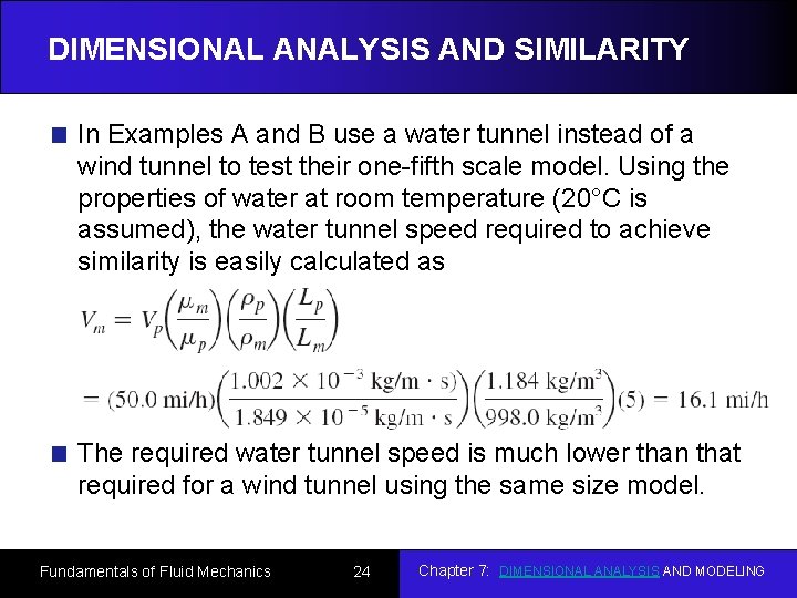
DIMENSIONAL ANALYSIS AND SIMILARITY In Examples A and B use a water tunnel instead of a wind tunnel to test their one-fifth scale model. Using the properties of water at room temperature (20°C is assumed), the water tunnel speed required to achieve similarity is easily calculated as The required water tunnel speed is much lower than that required for a wind tunnel using the same size model. Fundamentals of Fluid Mechanics 24 Chapter 7: DIMENSIONAL ANALYSIS AND MODELING

Method of Repeating Variables Nondimensional parameters can be generated by several methods. We will use the Method of Repeating Variables popularized by Edgar Buckingham (1867– 1940) and first published by the Russian scientist Dimitri Riabouchinsky (1882– 1962) in 1911. Six steps List the parameters in the problem and count their total number n. List the primary dimensions of each of the n parameters Set the reduction j as the number of primary dimensions. Calculate k, the expected number of ’s, k = n − j (Buckingham Pi theorem). Choose j repeating parameters. Construct the k ’s, and manipulate as necessary. Write the final functional relationship and check algebra. Fundamentals of Fluid Mechanics 25 Chapter 7: DIMENSIONAL ANALYSIS AND MODELING

Method of Repeating Variables The best way to learn the method is by example and practice. As we go through each step of the method of repeating variables, we explain some of the subtleties of the technique in more detail using the falling ball as an example. Fundamentals of Fluid Mechanics 26 Chapter 7: DIMENSIONAL ANALYSIS AND MODELING

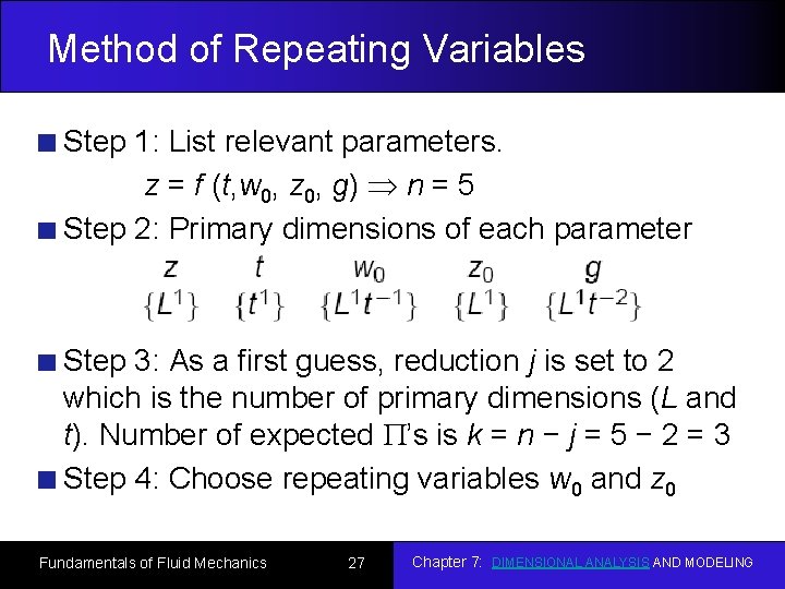
Method of Repeating Variables Step 1: List relevant parameters. z = f (t, w 0, z 0, g) n = 5 Step 2: Primary dimensions of each parameter Step 3: As a first guess, reduction j is set to 2 which is the number of primary dimensions (L and t). Number of expected ’s is k = n − j = 5 − 2 = 3 Step 4: Choose repeating variables w 0 and z 0 Fundamentals of Fluid Mechanics 27 Chapter 7: DIMENSIONAL ANALYSIS AND MODELING

Guidelines for choosing Repeating parameters Never pick the dependent variable. Otherwise, it may appear in all the ’s. Chosen repeating parameters must not by themselves be able to form a dimensionless group. Otherwise, it would be impossible to generate the rest of the ’s. Chosen repeating parameters must represent all the primary dimensions. Never pick parameters that are already dimensionless. Never pick two parameters with the same dimensions or with dimensions that differ by only an exponent. Choose dimensional constants over dimensional variables so that only one contains the dimensional variable. Pick common parameters since they may appear in each of the ’s. Pick simple parameters over complex parameters. Fundamentals of Fluid Mechanics 28 Chapter 7: DIMENSIONAL ANALYSIS AND MODELING

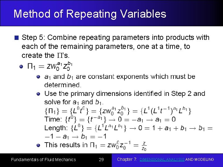
Method of Repeating Variables Step 5: Combine repeating parameters into products with each of the remaining parameters, one at a time, to create the ’s. Fundamentals of Fluid Mechanics 29 Chapter 7: DIMENSIONAL ANALYSIS AND MODELING

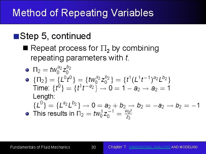
Method of Repeating Variables Step 5, continued Repeat process for 2 by combining repeating parameters with t. Fundamentals of Fluid Mechanics 30 Chapter 7: DIMENSIONAL ANALYSIS AND MODELING

Guidelines for manipulation of the ’s We may impose a constant (dimensionless) exponent on a or perform a functional operation on a . We may multiply a by a pure (dimensionless) constant. We may form a product (or quotient) of any with any other in the problem to replace one of the ’s. We may use any of guidelines 1 to 3 in combination. We may substitute a dimensional parameter in the with other parameter(s) of the same dimensions. Fundamentals of Fluid Mechanics 31 Chapter 7: DIMENSIONAL ANALYSIS AND MODELING

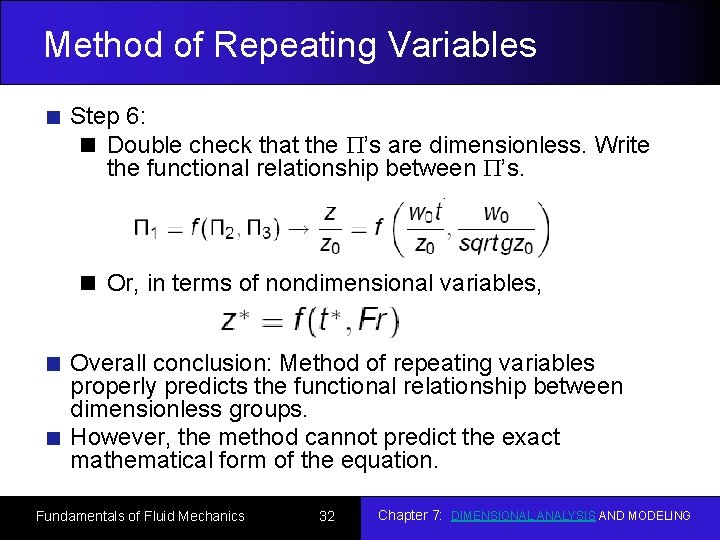
Method of Repeating Variables Step 6: Double check that the ’s are dimensionless. Write the functional relationship between ’s. Or, in terms of nondimensional variables, Overall conclusion: Method of repeating variables properly predicts the functional relationship between dimensionless groups. However, the method cannot predict the exact mathematical form of the equation. Fundamentals of Fluid Mechanics 32 Chapter 7: DIMENSIONAL ANALYSIS AND MODELING

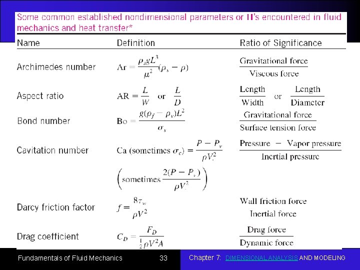
Fundamentals of Fluid Mechanics 33 Chapter 7: DIMENSIONAL ANALYSIS AND MODELING

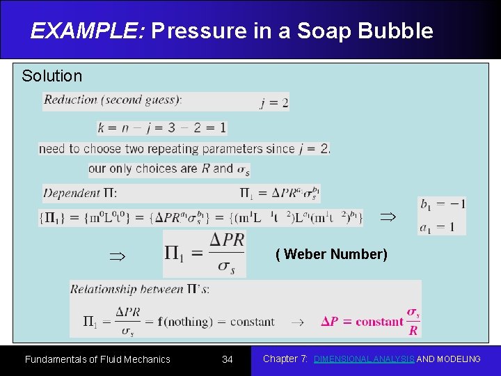
EXAMPLE: Pressure in a Soap Bubble Solution Consider the relationship between soap bubble radius and the pressure inside the soap bubble. The pressure inside the soap bubble must be greater than atmospheric pressure, and that the shell of the soap bubble is under tension, much like the skin of a balloon. You also know that the property surface tension must be important in this problem. Using dimensional analysis. Establish a( Weber Number) relationship between pressure difference soap bubble radius R, and the surface tension ss of the soap film. Fundamentals of Fluid Mechanics 34 Chapter 7: DIMENSIONAL ANALYSIS AND MODELING

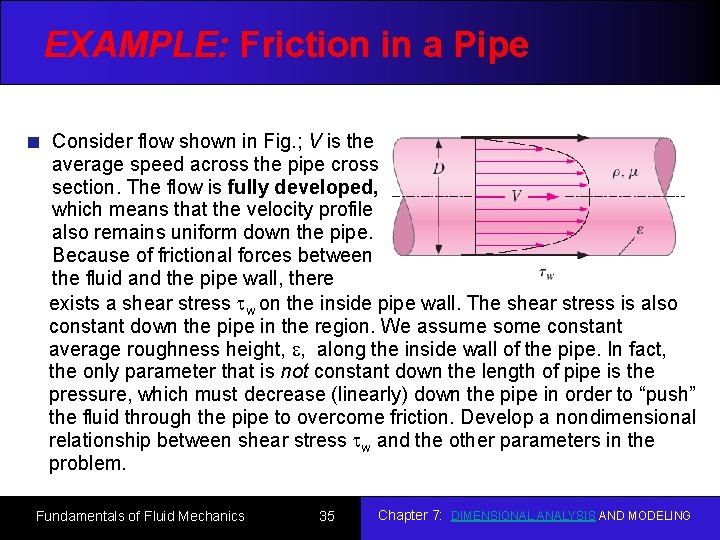
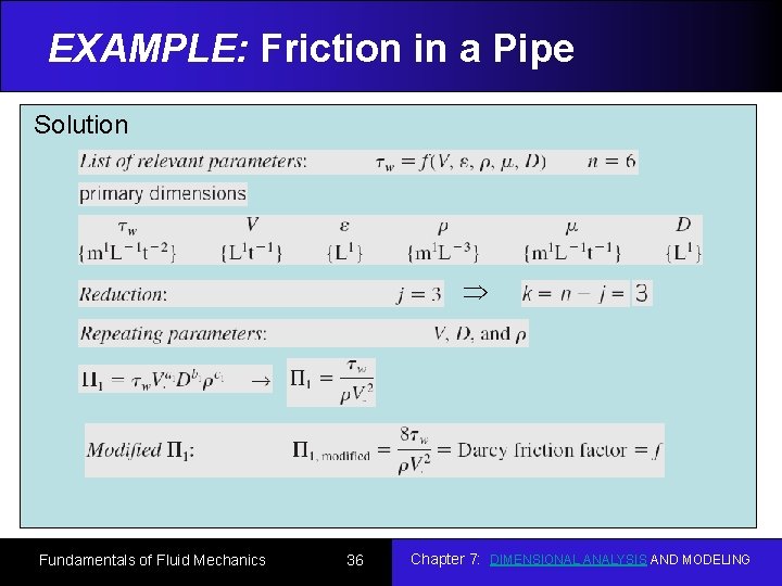
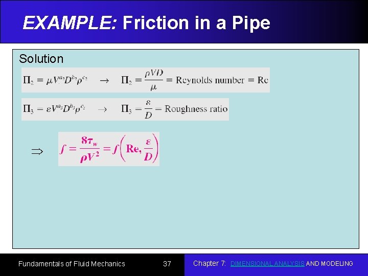
EXAMPLE: Friction in a Pipe Consider flow shown in Fig. ; V is the average speed across the pipe cross section. The flow is fully developed, which means that the velocity profile also remains uniform down the pipe. Because of frictional forces between the fluid and the pipe wall, there exists a shear stress tw on the inside pipe wall. The shear stress is also constant down the pipe in the region. We assume some constant average roughness height, , along the inside wall of the pipe. In fact, the only parameter that is not constant down the length of pipe is the pressure, which must decrease (linearly) down the pipe in order to “push” the fluid through the pipe to overcome friction. Develop a nondimensional relationship between shear stress tw and the other parameters in the problem. Fundamentals of Fluid Mechanics 35 Chapter 7: DIMENSIONAL ANALYSIS AND MODELING

EXAMPLE: Friction in a Pipe Solution Fundamentals of Fluid Mechanics 36 Chapter 7: DIMENSIONAL ANALYSIS AND MODELING

EXAMPLE: Friction in a Pipe Solution Fundamentals of Fluid Mechanics 37 Chapter 7: DIMENSIONAL ANALYSIS AND MODELING

Experimental Testing and Incomplete Similarity On of the most useful applications of dimensional analysis is in designing physical and or numerical experiments, and in reporting the results. Setup of an experiment and correlation of data Consider a problem with 5 parameters: one dependent and 4 independent. Full test matrix with 5 data points for each independent parameter would require 54 = 625 experiments!! If we can reduce to 2 ’s, the number of independent parameters is reduced from 4 to 1, which results in 51 = 5 experiments vs. 625!! Fundamentals of Fluid Mechanics 38 Chapter 7: DIMENSIONAL ANALYSIS AND MODELING

Experimental Testing and Incomplete Similarity Discussion of a two- problem, once the experiments are complete, plot ( 1) as a function of the independent dimensionless parameter ( 2). Then determine the functional form of the relationship by performing a regression analysis on the data. More than two ’s in the problem, need to set up a test matrix to determine the relationship between them. (How about only one Problem? ) Fundamentals of Fluid Mechanics 39 Chapter 7: DIMENSIONAL ANALYSIS AND MODELING

Experimental Testing and Incomplete Similarity It is not always possible to match all the ’s of a model to the corresponding ’s of the prototype. This situation is called incomplete similarity. Fortunately, in some cases of incomplete similarity, we are still able to extrapolate model tests to obtain reasonable full-scale predictions. Fundamentals of Fluid Mechanics 40 Chapter 7: DIMENSIONAL ANALYSIS AND MODELING

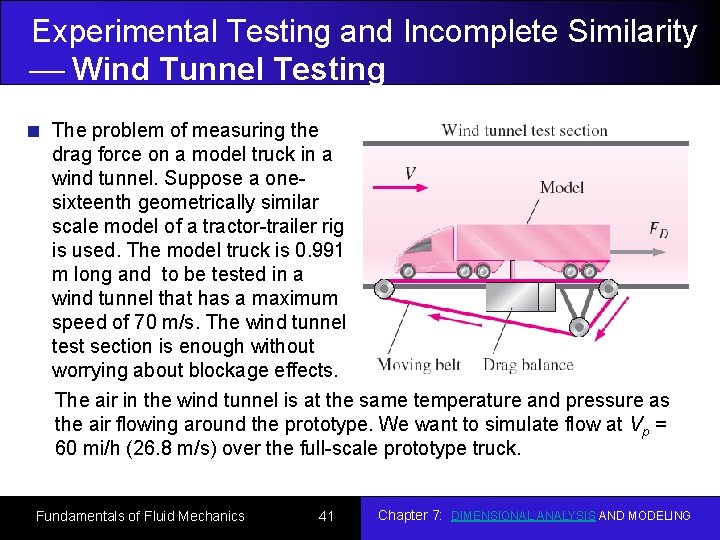
Experimental Testing and Incomplete Similarity Wind Tunnel Testing The problem of measuring the drag force on a model truck in a wind tunnel. Suppose a onesixteenth geometrically similar scale model of a tractor-trailer rig is used. The model truck is 0. 991 m long and to be tested in a wind tunnel that has a maximum speed of 70 m/s. The wind tunnel test section is enough without worrying about blockage effects. The air in the wind tunnel is at the same temperature and pressure as the air flowing around the prototype. We want to simulate flow at Vp = 60 mi/h (26. 8 m/s) over the full-scale prototype truck. Fundamentals of Fluid Mechanics 41 Chapter 7: DIMENSIONAL ANALYSIS AND MODELING

Experimental Testing and Incomplete Similarity Wind Tunnel Testing The first thing we do is match the Reynolds numbers, The required wind tunnel speed for the model tests Vm is This speed is more than six times greater than the maximum achievable wind tunnel speed. Also, the flow would be supersonic (about 346 m/s). While the Mach number of the prototype ( 0. 080) does not match the Mach number of the model (1. 28). It is clearly not possible to match the model Reynolds number to that of the prototype with this model and wind tunnel facility. What do we do? Fundamentals of Fluid Mechanics 42 Chapter 7: DIMENSIONAL ANALYSIS AND MODELING

Experimental Testing and Incomplete Similarity Wind Tunnel Testing Several options to resolve the incomplete similarity: Use a bigger wind tunnel. (Automobile manufacturers typically test with 3/8 scale model cars and with 1/8 scale model trucks and buses in very large wind tunnels. ) However, it is more expensive. How big can a model be? A useful rule of thumb is that the blockage (ratio of the model frontal area to the cross sectional area of the test section) should be less than 7. 5 percent. Use a different fluid for the model tests. Water tunnels can achieve higher Reynolds numbers than can wind tunnels of the same size, but they are much more expensive to build and operate. Pressurize the wind tunnel and/or adjust the air temperature to increase the maximum Reynolds number capability (limited). Run the wind tunnel at several speeds near the maximum speed, and then extrapolate our results to the full-scale Reynolds number. Fundamentals of Fluid Mechanics 43 Chapter 7: DIMENSIONAL ANALYSIS AND MODELING

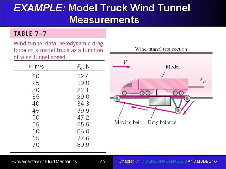
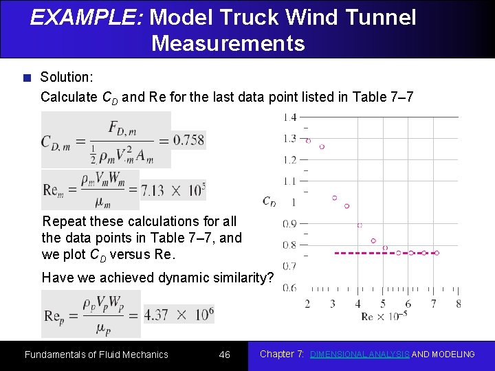
EXAMPLE: Model Truck Wind Tunnel Measurements A one-sixteenth scale model tractor-trailer truck is tested in a wind tunnel. The model truck is 0. 991 m long, 0. 257 m tall, and 0. 159 m wide. Aerodynamic drag force FD is measured as a function of wind tunnel speed; the experimental results are listed in Table 7– 7. Plot the drag coefficient CD as a function of Re, where the area used for the calculation of CD is the frontal area of the model truck, and the length scale used for calculation of Re is truck width W. Have we achieved dynamic similarity? Have we achieved Reynolds number independence in our wind tunnel test? Estimate the aerodynamic drag force on the prototype truck traveling on the highway at 26. 8 m/s. Assume that both the wind tunnel air and the air flowing over the prototype car are at 25°C and standard atmospheric pressure. Fundamentals of Fluid Mechanics 44 Chapter 7: DIMENSIONAL ANALYSIS AND MODELING

EXAMPLE: Model Truck Wind Tunnel Measurements Fundamentals of Fluid Mechanics 45 Chapter 7: DIMENSIONAL ANALYSIS AND MODELING

EXAMPLE: Model Truck Wind Tunnel Measurements Solution: Calculate CD and Re for the last data point listed in Table 7– 7 Repeat these calculations for all the data points in Table 7– 7, and we plot CD versus Re. Have we achieved dynamic similarity? Fundamentals of Fluid Mechanics 46 Chapter 7: DIMENSIONAL ANALYSIS AND MODELING

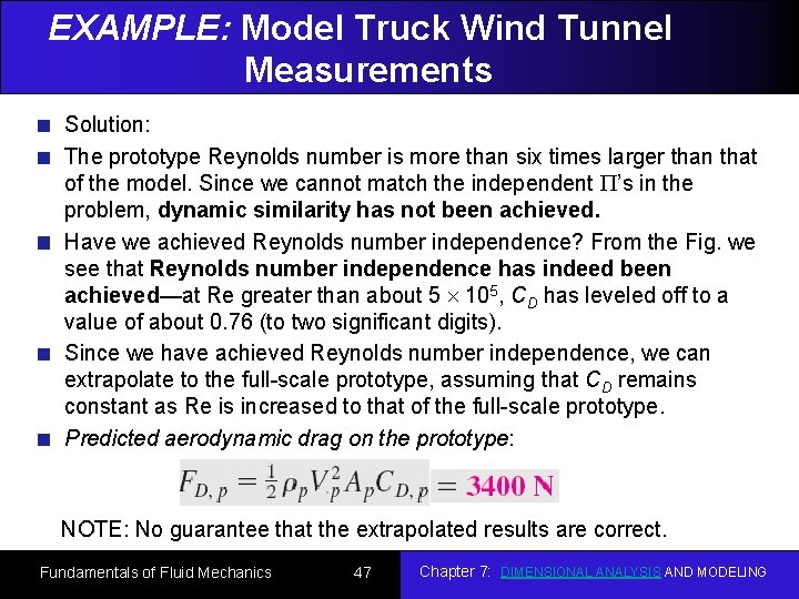
EXAMPLE: Model Truck Wind Tunnel Measurements Solution: The prototype Reynolds number is more than six times larger than that of the model. Since we cannot match the independent ’s in the problem, dynamic similarity has not been achieved. Have we achieved Reynolds number independence? From the Fig. we see that Reynolds number independence has indeed been achieved—at Re greater than about 5 105, CD has leveled off to a value of about 0. 76 (to two significant digits). Since we have achieved Reynolds number independence, we can extrapolate to the full-scale prototype, assuming that CD remains constant as Re is increased to that of the full-scale prototype. Predicted aerodynamic drag on the prototype: NOTE: No guarantee that the extrapolated results are correct. Fundamentals of Fluid Mechanics 47 Chapter 7: DIMENSIONAL ANALYSIS AND MODELING

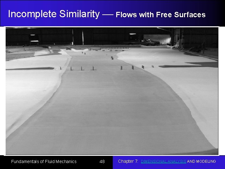
Incomplete Similarity Flows with Free Surfaces For the case of model testing of flows with free surfaces (boats and ships, floods, river flows, aqueducts, hydroelectric dam spillways, interaction of waves with piers, soil erosion, etc. ), complications arise that preclude complete similarity between model and prototype. For example, if a model river is built to study flooding, the model is often several hundred times smaller than the prototype due to limited lab space. This may cause, for instance, Increase the effect of surface tension Turbulent flow laminar flow To avoid these problems, researchers often use a distorted model in which the vertical scale of the model (e. g. , river depth) is exaggerated in comparison to the horizontal scale of the model (e. g. , river width). Fundamentals of Fluid Mechanics 48 Chapter 7: DIMENSIONAL ANALYSIS AND MODELING

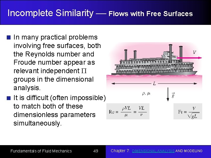
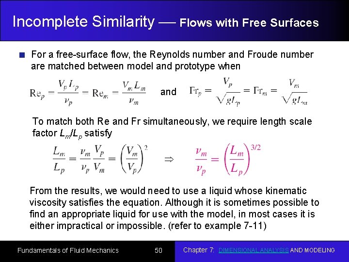
Incomplete Similarity Flows with Free Surfaces In many practical problems involving free surfaces, both the Reynolds number and Froude number appear as relevant independent groups in the dimensional analysis. It is difficult (often impossible) to match both of these dimensionless parameters simultaneously. Fundamentals of Fluid Mechanics 49 Chapter 7: DIMENSIONAL ANALYSIS AND MODELING

Incomplete Similarity Flows with Free Surfaces For a free-surface flow, the Reynolds number and Froude number are matched between model and prototype when and To match both Re and Fr simultaneously, we require length scale factor Lm/Lp satisfy From the results, we would need to use a liquid whose kinematic viscosity satisfies the equation. Although it is sometimes possible to find an appropriate liquid for use with the model, in most cases it is either impractical or impossible. (refer to example 7 -11) Fundamentals of Fluid Mechanics 50 Chapter 7: DIMENSIONAL ANALYSIS AND MODELING