FUNDAMENTALS OF FINITE VOLUME METHODS FLUID A substance

FUNDAMENTALS OF FINITE VOLUME METHODS

FLUID? • A substance in the liquid or gas phase is referred to as a fluid. • In fluids, stress is proportional to strain rate. • Fluid never stops deforming and approaches a constant rate of strain. • A fluid at rest, the normal stress is called pressure. • A fluid at rest is at a state of zero shear stress.

CLASSIFICATION OF FLUID FLOWS • Viscous versus Inviscid Regions of Flow • Internal versus External Flow • Compressible versus Incompressible Flow • Laminar versus Turbulent Flow • Natural (or Unforced) versus Forced Flow • Steady versus Unsteady Flow • One-, Two-, and Three-Dimensional Flows

NO-SLIP CONDITION

Laminar flow is encountered when LAMINAR AND highly viscous fluids such as oils flow TURBULENT FLOWS in small pipes or narrow passages. Laminar: Smooth streamlines and highly ordered motion. Turbulent: Velocity fluctuations and highly disordered motion. Transition: The flow fluctuates between laminar and turbulent flows. Most flows encountered in practice are turbulent. Laminar and regimes of and turbulent flow . motion The behavior of colored fluid injected into the candle smoke flow in laminar flows in a pipe. flow in laminar 6

FLUID FLOW IN PIPES • The Reynolds number Re is the ratio of the inertia forces in the flow to the viscous forces in the flow and can be calculated using: • • If Re < 2000, the flow will be laminar. If Re > 4000, the flow will be turbulent. If 2000<Re<4000, the flow is transitional The Reynolds number is a good guide to the type of flow

FLUID FLOW IN PIPES

DIFFERENTIAL ANALYSIS OF FLUID FLOW • Involves application of differential equations of fluid motion to any and every point in the flow field over a region called the flow domain. • Differential technique as the analysis of millions of tiny control volumes stacked end to end and on top of each other all throughout the flow field. • In the limit as the number of tiny control volumes goes to infinity, and the size of each control volume shrinks to a point, the conservation equations simplify to a set of partial differential equations that are valid at any point in the flow. • When solved, these differential equations yield details about the velocity, density, pressure, etc. , at every point throughout the entire flow domain. • For three-dimensional incompressible flow, there are four unknowns (velocity components u, v, w, and pressure P) and four equations (one from conservation of mass, which is a scalar equation, and three from Newton’s second law, which is a vector equation).

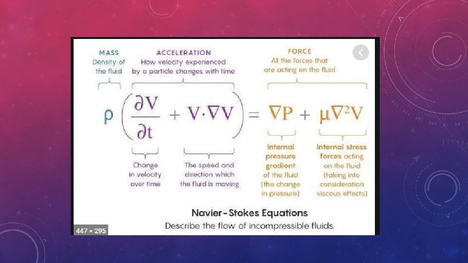
NAVIER–STOKES EQUATIONS • Differential equations of fluid motion Namely, conservation of mass (the continuity equation) and Newton’s second law (the Navier–Stokes equation) • Equations apply to every point in the flow field and thus enable us to solve for all details of the flow everywhere in the flow domain.

RECALLING VECTOR OPERATIONS • Del Operator: • Laplacian Operator: • Gradient: l Vector Gradient: l Divergence: l Directional Derivative:

MOMENTUM CONSERVATION y z x

EULER’S EQUATIONS Note: Integration of the Euler’s equations along a streamline will give rise to the Bernoulli’s equation.

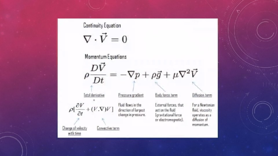
CONTINUITY EQUATION FOR INCOMPRESSIBLE (CONSTANT DENSITY) FLOW - derived from conservation of mass where u is the velocity vector u, v, w are velocities in x, y, and z directions

NAVIER-STOKES EQUATION FOR INCOMPRESSIBLE FLOW OF NEWTONIAN (CONSTANT VISCOSITY) FLUID - derived from conservation of momentum υ kinematic viscosity (constant) density (constant) ρ pressure external force (such as gravity)

NAVIER-STOKES EQUATION FOR INCOMPRESSIBLE FLOW OF NEWTONIAN (CONSTANT VISCOSITY) FLUID - derived from conservation of momentum υ υ ρ ρ

NAVIER-STOKES EQUATION FOR INCOMPRESSIBLE FLOW OF NEWTONIAN (CONSTANT VISCOSITY) FLUID - derived from conservation of momentum υ Acceleration term: change of velocity with time ρ

NAVIER-STOKES EQUATION FOR INCOMPRESSIBLE FLOW OF NEWTONIAN (CONSTANT VISCOSITY) FLUID - derived from conservation of momentum υ Advection term: force exerted on a particle of fluid by the other particles of fluid surrounding it ρ

NAVIER-STOKES EQUATION FOR INCOMPRESSIBLE FLOW OF NEWTONIAN (CONSTANT VISCOSITY) FLUID - derived from conservation of momentum υ ρ viscosity (constant) controlled velocity diffusion term: (this term describes how fluid motion is damped) • Highly viscous fluids stick together (honey) • Low-viscosity fluids flow freely (air)

NAVIER-STOKES EQUATION FOR INCOMPRESSIBLE FLOW OF NEWTONIAN (CONSTANT VISCOSITY) FLUID - derived from conservation of momentum υ ρ Pressure term: Fluid flows in the direction of largest change in pressure

NAVIER-STOKES EQUATION FOR INCOMPRESSIBLE FLOW OF NEWTONIAN (CONSTANT VISCOSITY) FLUID - derived from conservation of momentum υ ρ Body force term: external forces that act on the fluid (such as gravity, electromagnetic, etc. )

NAVIER-STOKES EQUATION FOR INCOMPRESSIBLE FLOW OF NEWTONIAN (CONSTANT VISCOSITY) FLUID - derived from conservation of momentum υ ρ change body in = advection + diffusion + pressure + force velocity with time

EQUATIONS FOR INCOMPRESSIBLE FLOW OF NEWTONIAN FLUID υ ρ

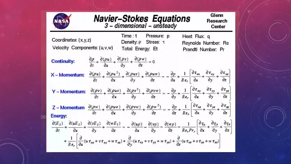
CONTINUITY AND NAVIER-STOKES EQUATIONS FOR INCOMPRESSIBLE FLOW OF NEWTONIAN FLUID in Cartesian coordinates Continuity: Navier-Stokes: x - component: y - component: z - component:

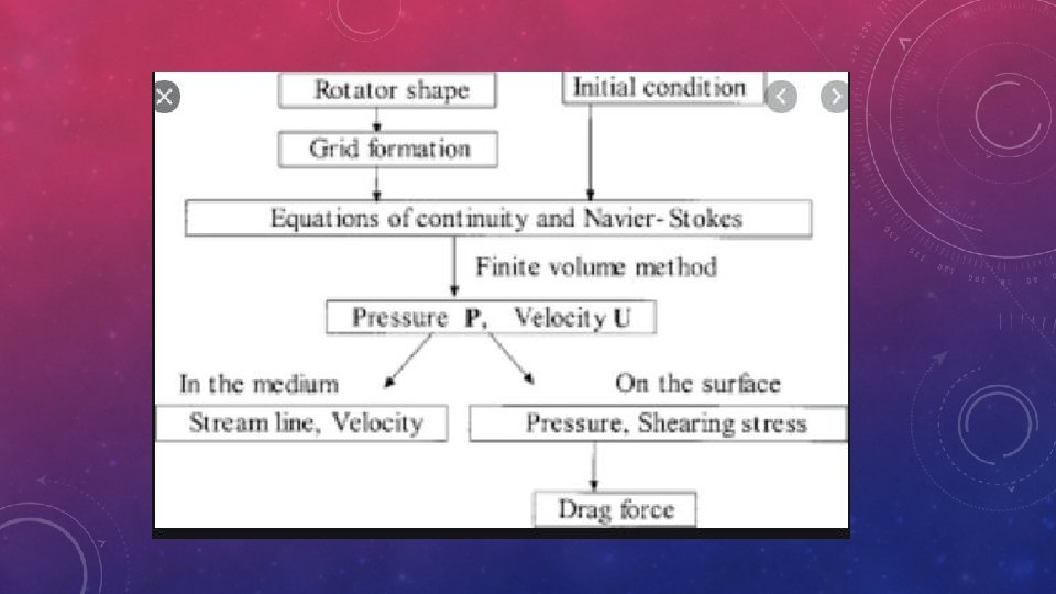
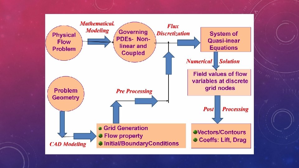
Finite volume method (FVM) • • • ▪ A finite volume method (FVM) discretization is based upon an integral form of the PDE to be solved (e. g. conservation of mass, momentum, or energy). The PDE is written in a form which can be solved for a given finite volume (or cell). The computational domain is discretized into finite volumes and then for every volume the governing equations are solved. The resulting system of equations usually involves fluxes of the conserved variable, and thus the calculation of fluxes is very important in FVM. The basic advantage of this method over FDM is it does not require the use of structured grids, and the effort to convert the given mesh in to structured numerical grid internally is completely avoided. As with FDM, the resulting approximate solution is a discrete, but the variables are typically placed at cell centers rather than at nodal points. This is not always true, as there also face-centered finite volume methods. In any case, the values of field variables at non-storage locations (e. g. vertices) are obtained using interpolation.