Fundamental Techniques 1 Divide and Conquer 2 Dynamic

Fundamental Techniques 1. Divide and Conquer 2. Dynamic Programming 3. Greedy Algorithm

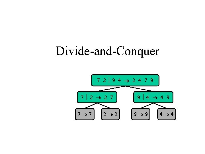
Divide-and-Conquer 7 2 9 4 2 4 7 9 7 2 2 7 7 7 2 2 9 4 4 9 9 9 4 4

Divide-and-Conquer • Divide-and conquer is a general algorithm design paradigm: – Divide: divide the input data S in two or more disjoint subsets S 1, S 2, … – Recur: solve the subproblems recursively – Conquer: combine the solutions for S 1, S 2, …, into a solution for S • The base case for the recursion are subproblems of constant size • Analysis can be done using recurrence equations

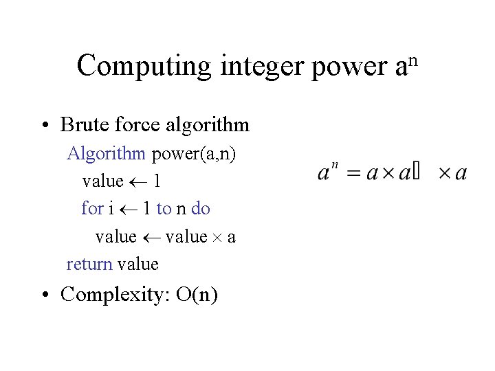
Computing integer power • Brute force algorithm Algorithm power(a, n) value 1 for i 1 to n do value a return value • Complexity: O(n) n a

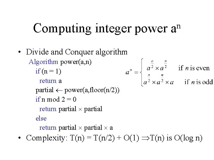
Computing integer power n a • Divide and Conquer algorithm Algorithm power(a, n) if (n = 1) return a partial power(a, floor(n/2)) if n mod 2 = 0 return partial else return partial a • Complexity: T(n) = T(n/2) + O(1) T(n) is O(log n)

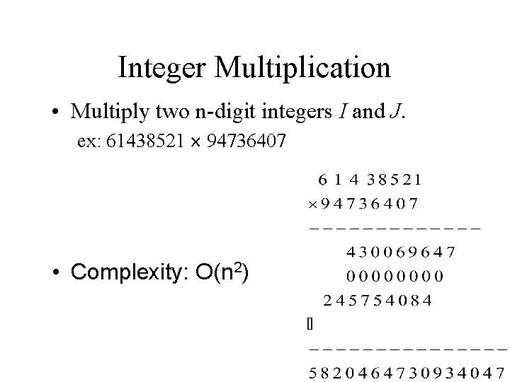
Integer Multiplication • Multiply two n-digit integers I and J. ex: 61438521 94736407 • Complexity: O(n 2)

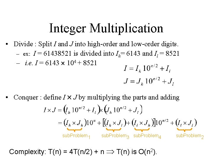
Integer Multiplication • Divide : Split I and J into high-order and low-order digits. – ex: I = 61438521 is divided into Ih= 6143 and Il = 8521 – i. e. I = 6143 104 + 8521 • Conquer : define I J by multiplying the parts and adding sub. Problem 1 sub. Problem 3 sub. Problem 4 Complexity: T(n) = 4 T(n/2) + n T(n) is O(n 2). sub. Problem 2

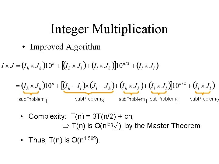
Integer Multiplication • Improved Algorithm sub. Problem 1 sub. Problem 3 sub. Problem 1 sub. Problem 2 • Complexity: T(n) = 3 T(n/2) + cn, T(n) is O(nlog 23), by the Master Theorem • Thus, T(n) is O(n 1. 585).

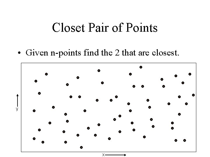
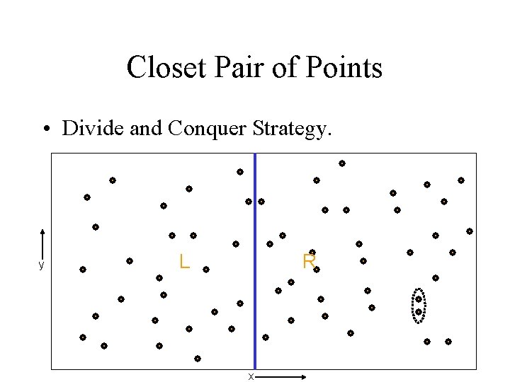
Closet Pair of Points • Given n-points find the 2 that are closest. y x

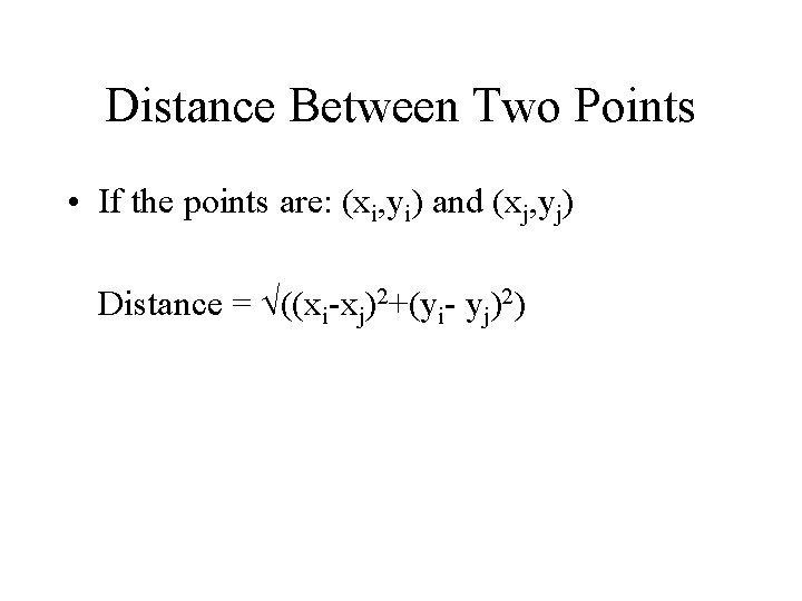
Distance Between Two Points • If the points are: (xi, yi) and (xj, yj) Distance = ((xi-xj)2+(yi- yj)2)

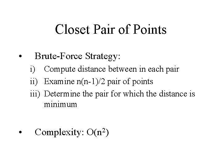
Closet Pair of Points • Brute-Force Strategy: i) Compute distance between in each pair ii) Examine n(n-1)/2 pair of points iii) Determine the pair for which the distance is minimum • Complexity: O(n 2)

Closet Pair of Points • Divide and Conquer Strategy. y L R x

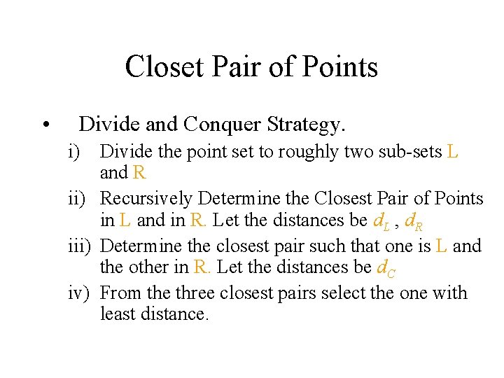
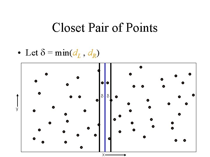
Closet Pair of Points • Divide and Conquer Strategy. i) Divide the point set to roughly two sub-sets L and R ii) Recursively Determine the Closest Pair of Points in L and in R. Let the distances be d. L , d. R iii) Determine the closest pair such that one is L and the other in R. Let the distances be d. C iv) From the three closest pairs select the one with least distance.

Closet Pair of Points • Let = min(d. L , d. R) y x

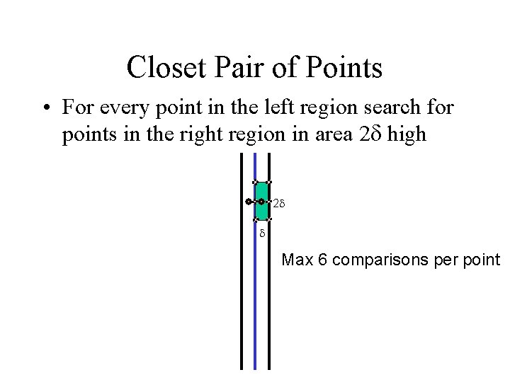
Closet Pair of Points • For every point in the left region search for points in the right region in area 2 high 2 Max 6 comparisons per point

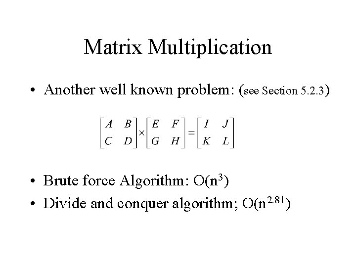
Matrix Multiplication • Another well known problem: (see Section 5. 2. 3) • Brute force Algorithm: O(n 3) • Divide and conquer algorithm; O(n 2. 81)

Dynamic Programming

Dynamic Algorithm • Most difficult of the fundamental techniques. [Ref: Sahni, “Data Structure and Algorithms and Applications”] • Takes a problem that seems to require exponential time and produces polynomial-time algorithm to solve it. • The resulting algorithm is simple. Often requires a few lines of code.

Recursive Algorithms • Best when sub-problems are disjoint. • Example of Inefficient Recursive Algorithm: Fibonacci Number: F(n) = F(n-1) + F(n-2)

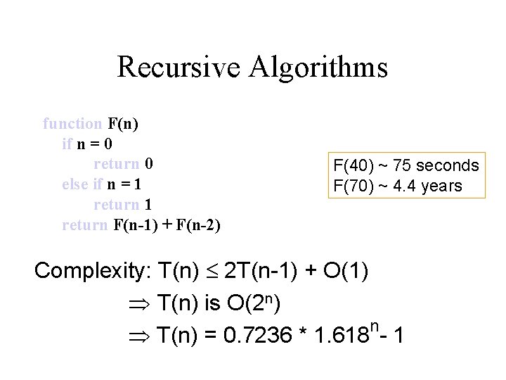
Recursive Algorithms function F(n) if n = 0 return 0 else if n = 1 return F(n-1) + F(n-2) F(40) ~ 75 seconds F(70) ~ 4. 4 years Complexity: T(n) 2 T(n-1) + O(1) T(n) is O(2 n) n T(n) = 0. 7236 * 1. 618 - 1

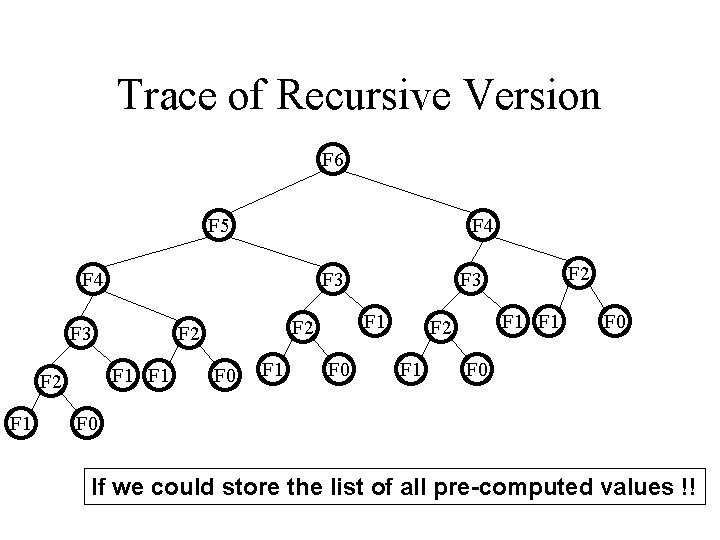
Trace of Recursive Version F 6 F 5 F 4 F 3 F 1 F 1 F 2 F 2 F 0 F 1 F 0 F 2 F 3 F 1 F 2 F 1 F 0 F 0 If we could store the list of all pre-computed values !!

Dynamic Programming • Find a recursive solution that involves solving the same problem many times. • Calculate bottom up and avoid recalculation

Efficient Version • Linear Time Iterative: Algorithm Fibonacci(n) Fn[0] 0 Fn[1] 1 for i 2 to n do Fn[i] Fn[i-1] + Fn[i-2] return Fn[n] Fibonacci(40) < microseconds Fibonacci(70) < microseconds

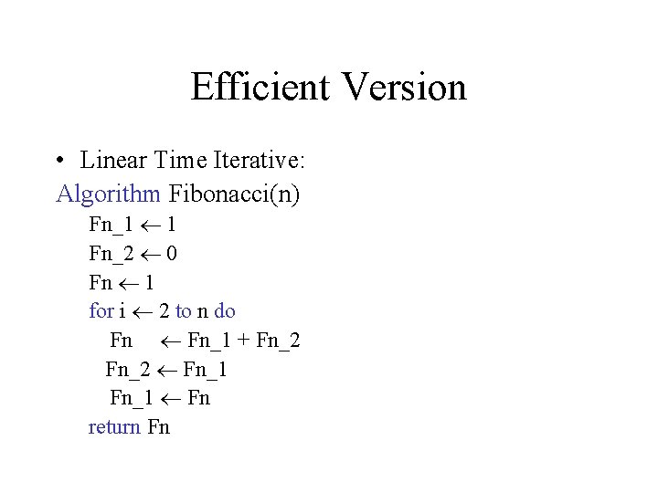
Efficient Version • Linear Time Iterative: Algorithm Fibonacci(n) Fn_1 1 Fn_2 0 Fn 1 for i 2 to n do Fn Fn_1 + Fn_2 Fn_1 Fn return Fn

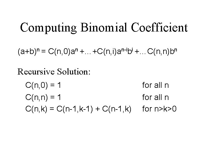
Computing Binomial Coefficient (a+b)n = C(n, 0)an +…+C(n, i)an-ibi +…C(n, n)bn Recursive Solution: C(n, 0) = 1 C(n, n) = 1 C(n, k) = C(n-1, k-1) + C(n-1, k) for all n for n>k>0

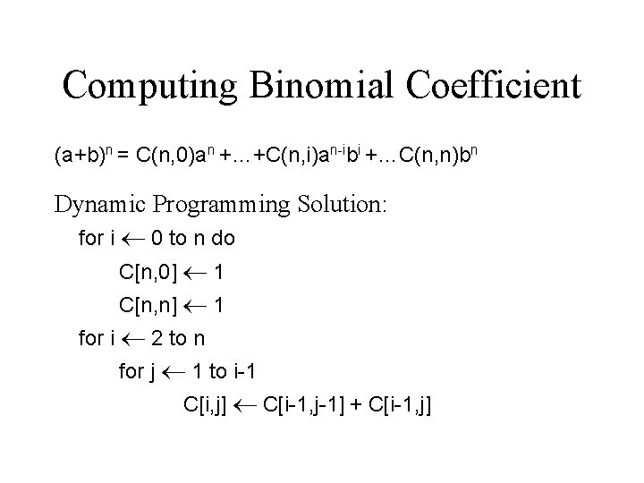
Computing Binomial Coefficient (a+b)n = C(n, 0)an +…+C(n, i)an-ibi +…C(n, n)bn Dynamic Programming Solution: for i 0 to n do C[n, 0] 1 C[n, n] 1 for i 2 to n for j 1 to i-1 C[i, j] C[i-1, j-1] + C[i-1, j]

Dynamic Programming • Best used for solving optimization problems. • Optimization Problem defn: – Many solutions possible – Choose a solution that minimizes the cost

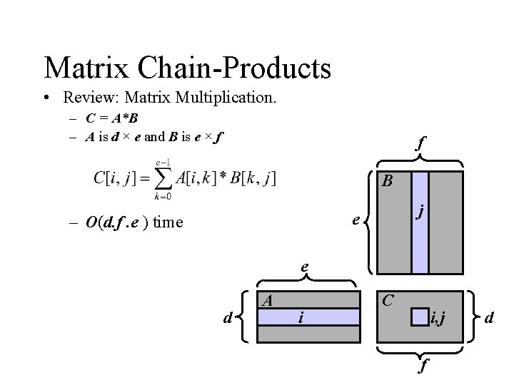
Matrix Chain-Products • Review: Matrix Multiplication. – C = A*B – A is d × e and B is e × f f B j e – O(d. f. e ) time e d A i C i, j f d

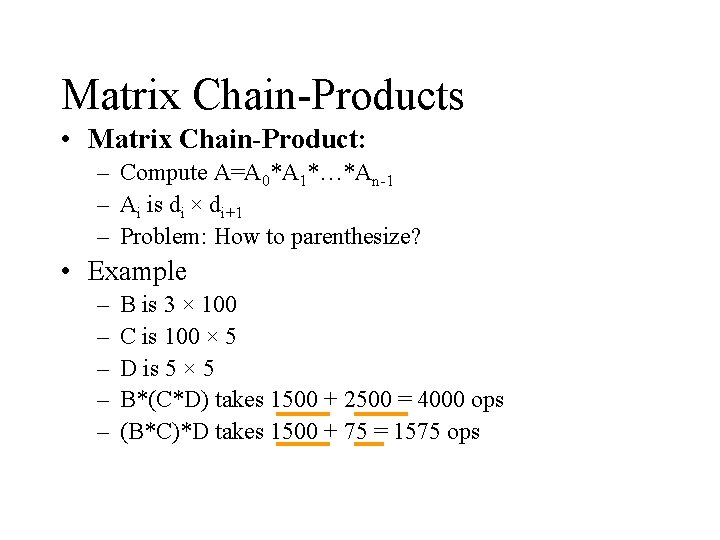
Matrix Chain-Products • Matrix Chain-Product: – Compute A=A 0*A 1*…*An-1 – Ai is di × di+1 – Problem: How to parenthesize? • Example – – – B is 3 × 100 C is 100 × 5 D is 5 × 5 B*(C*D) takes 1500 + 2500 = 4000 ops (B*C)*D takes 1500 + 75 = 1575 ops

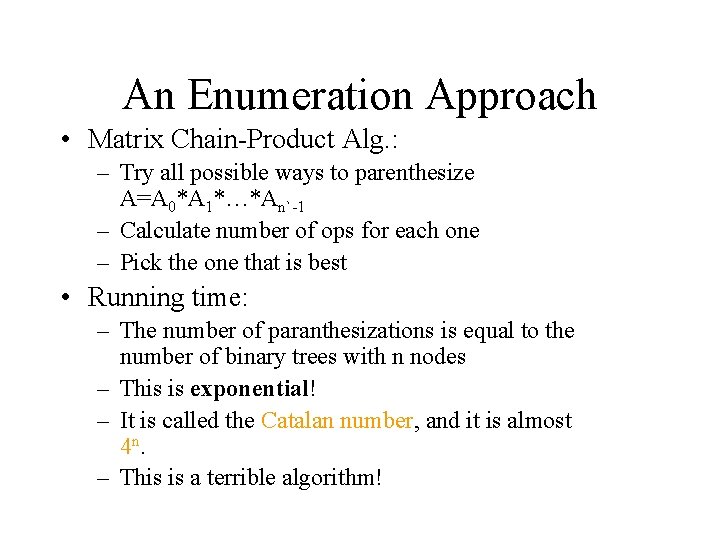
An Enumeration Approach • Matrix Chain-Product Alg. : – Try all possible ways to parenthesize A=A 0*A 1*…*An`-1 – Calculate number of ops for each one – Pick the one that is best • Running time: – The number of paranthesizations is equal to the number of binary trees with n nodes – This is exponential! – It is called the Catalan number, and it is almost 4 n. – This is a terrible algorithm!

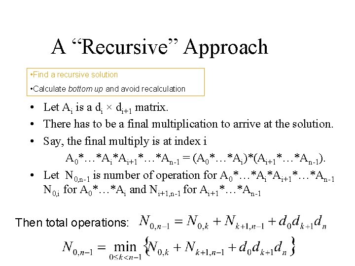
A “Recursive” Approach • Find a recursive solution • Calculate bottom up and avoid recalculation • Let Ai is a di × di+1 matrix. • There has to be a final multiplication to arrive at the solution. • Say, the final multiply is at index i A 0*…*Ai*Ai+1*…*An-1 = (A 0*…*Ai)*(Ai+1*…*An-1). • Let N 0, n-1 is number of operation for A 0*…*Ai*Ai+1*…*An-1 N 0, i for A 0*…*Ai and Ni+1, n-1 for Ai+1*…*An-1 Then total operations:

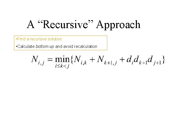
A “Recursive” Approach • Find a recursive solution • Calculate bottom up and avoid recalculation

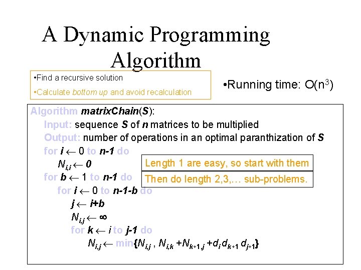
A Dynamic Programming Algorithm • Find a recursive solution • Calculate bottom up and avoid recalculation • Running time: O(n 3) Algorithm matrix. Chain(S): Input: sequence S of n matrices to be multiplied Output: number of operations in an optimal paranthization of S for i 0 to n-1 do Length 1 are easy, so start with them Ni, i 0 for b 1 to n-1 do Then do length 2, 3, … sub-problems. for i 0 to n-1 -b do j i+b Ni, j for k i to j-1 do Ni, j min{Ni, j , Ni, k +Nk+1, j +di dk+1 dj+1}

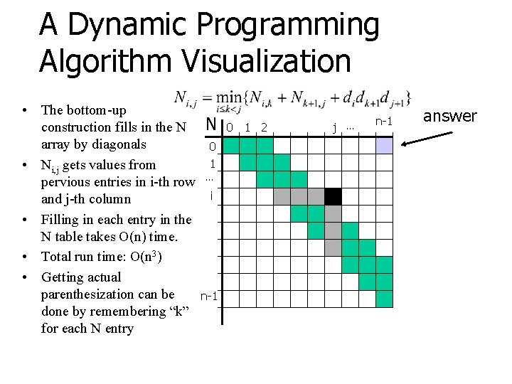
A Dynamic Programming Algorithm Visualization • The bottom-up construction fills in the N N array by diagonals 0 1 • Ni, j gets values from pervious entries in i-th row … i and j-th column • Filling in each entry in the N table takes O(n) time. • Total run time: O(n 3) • Getting actual parenthesization can be n-1 done by remembering “k” for each N entry 0 1 2 j … n-1 answer

Dynamic Programming • Is based on Principle of Optimality • Generally reduces the complexity of exponential problem to polynomial problem • Often computes data for all feasible solutions, but stores the data and reuses

When to Use Dynamic Programming? • Brute Force solution is prohibitively expensive • Problem must be divisible into multiple stages • Choices made at each stage include the choices made at previous stages.