Fundamental Algorithms Chapter 4 Shortest Paths Sevag Gharibian

Fundamental Algorithms Chapter 4: Shortest Paths Sevag Gharibian (based on slides of Christian Scheideler) WS 2018

Shortest Paths t s Central question: Determine fastest way to get from s to t. 31. 10. 2020 Chapter 4 2

Shortest Paths Shortest Path Problem: • directed/undirected graph G=(V, E) • edge costs c: E ℝ • SSSP (single source shortest path): find shortest paths from a source node to all other nodes – In Lecture 2, we solved this using Dijkstra‘s algorithm and Priority Queues. – Q: What is different about the setting here? • APSP (all pairs shortest path): find shortest paths between all pairs of nodes 31. 10. 2020 Chapter 4 3

Shortest Paths 42 0 - 5 - -1 0 + - - 2 2 0 s 0 -2 -3 -1 -2 -3 (s, v): distance between s and v no path from s to v (s, v) = - path of arbitrarily low cost from s to v min{ c(p) | p is a path from s to v} 31. 10. 2020 Chapter 4 4

Shortest Paths 42 0 - 5 - -1 0 + - 0 -2 -3 2 0 s - 2 -1 -2 -3 When is the distance - ? If there is a negative cycle: s 31. 10. 2020 C v Chapter 4 c(C)<0 5

Shortest Paths Negative cycle necessary and sufficient for a distance of -. Negative cycle sufficient: s path p path q C v c(C)<0 Cost for i-fold traversal of C: c(p) + i c(C) + c(q) For i this expression approaches -. 31. 10. 2020 Chapter 4 6

Shortest Paths Negative cycle necessary and sufficient for a distance of -. Negative cycle necessary: • l: minimal cost of a simple path from s to v • suppose there is a non-simple path p from s to v with cost c(r)<l • p non-simple: continuously remove a cycle C till we are left with a simple path • since c(p) < l, there must be a cycle C with c(C)<0 31. 10. 2020 Chapter 4 7

Shortest Paths in Arbitrary Graphs General Strategy: • Initially, set d(s): =0 and d(v): = for all other nodes • For every visited v, update distances to nodes w with (v, w) E, i. e. , d(w): = min{d(w), d(v)+c(v, w)} • But what order to visit the edges E in? 31. 10. 2020 Chapter 4 8

Bellman-Ford Algorithm Consider graphs with arbitrary (real) edge costs. Problem: visit nodes along a shortest path from s to v in the „right order“ s w 0 d 1 d 2 d 3 d 4 v Dijkstra´s algorithm cannot be used in this case any more – let‘s do an example to see why. 31. 10. 2020 Chapter 4 9

Bellman-Ford Algorithm Example (Dijkstra with negative weights): v 2 0 2 -1 1 s 3 3 -1 1 -4 Node v has wrong distance value! (Why? ) 31. 10. 2020 Chapter 4 10

Bellman-Ford Algorithm Lemma 4. 1: For every node v with (s, v)>- there is a simple path (without cycle!) from s to v of length (s, v). Proof: • Path with cycle of length 0: removing the cycle does not increase the path length • Path with cycle of length <0: distance from s is - ! 31. 10. 2020 Chapter 4 11

Bellman-Ford Algorithm Conclusion: (graph with n nodes) For every node v with (s, v)> - there is a shortest path along <n nodes to v. Why is this important? • It gives us a stopping criterion. • Namely, takes at most n-1 steps to compute (s, v). 31. 10. 2020 Chapter 4 12

Bellman-Ford Algorithm Conclusion: (graph with n nodes) For every node v with (s, v)> - there is a shortest path along <n nodes to v. Strategy: repeat the following n-1 times – for each edge e in E, traverse e and update relevant node costs. Claim: This will consider all simple paths of length n-1. 31. 10. 2020 Chapter 4 13

Bellman-Ford Algorithm Strategy: repeat the following n-1 times – for each edge e in E, traverse e and update relevant node costs. Claim: This will consider all simple paths of length n-1. Why? Proof sketch: For any simple path p, let ei be its ith edge. Then, we view round i of the iteration as traversing edge ei. 31. 10. 2020 Chapter 4 14

Bellman-Ford Algorithm Proof sketch: For any simple path p, ei be its ith edge. Then, we view round i of the loop as traversing edge ei. – Another viewpoint: Each iteration „applies all edges in parallel“. Aside: This idea is used in other places, too – e. g. , if A is the adjacency matrix of a graph, then entry (i, j) of An contains number of walks of length n from vertex i to vertex j. 31. 10. 2020 Chapter 4 15

Bellman-Ford Algorithm Problem: detection of negative cycles -2 1 s 1 0 1 -1 1 1 0 2 -1 Conclusion: in a negative cycle, distance of at least one node keeps decreasing in each round, starting with a round <n 31. 10. 2020 Chapter 4 16

Bellman-Ford Algorithm Lemma 4. 2: • If no decrease of a distance in a round (i. e. , d[v]+c(v, w)≥d[w] for all w), then d[w]= (s, w) for all w (i. e. reached correct values) • If some node w‘s distance decreases in n-th round (i. e. , d[v]+c(v, w)<d[w] for some w): There are negative cycles for all such w, so node w has distance (s, w)=-. If this is true for w, then also for all nodes reachable from w. Proof: exercise 31. 10. 2020 Chapter 4 17

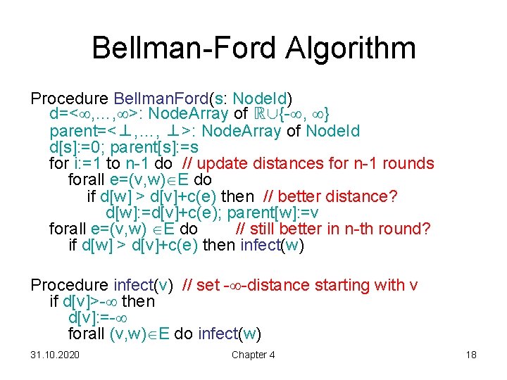
Bellman-Ford Algorithm Procedure Bellman. Ford(s: Node. Id) d=< , …, >: Node. Array of ℝ∪{- , } parent=<⊥, …, ⊥>: Node. Array of Node. Id d[s]: =0; parent[s]: =s for i: =1 to n-1 do // update distances for n-1 rounds forall e=(v, w) E do if d[w] > d[v]+c(e) then // better distance? d[w]: =d[v]+c(e); parent[w]: =v forall e=(v, w) E do // still better in n-th round? if d[w] > d[v]+c(e) then infect(w) Procedure infect(v) // set - -distance starting with v if d[v]>- then d[v]: =- forall (v, w) E do infect(w) 31. 10. 2020 Chapter 4 18

Bellman-Ford Algorithm Runtime: O(n m) Improvements: • Check in each update round if we still have d[v]+c[v, w]<d[w] for some (v, w) E. No: done! • Visit in each round only those nodes w with some edge (v, w) E where d[v] has decreased in the previous round. 31. 10. 2020 Chapter 4 19

All Pairs Shortest Paths Assumption: graph with arbitrary edge costs, but no negative cycles Naive Strategy for a graph with n nodes: run n times Bellman-Ford Algorithm (once for every node as the source) Runtime: O(n 2 m) 31. 10. 2020 Chapter 4 20

All Pairs Shortest Paths Better Strategy: Reduce n Bellman-Ford applications to n Dijkstra applications (Recall: Dijkstra requires O((m+n)logn) time using binary heaps. ) Problem: we need non-negative edge costs Solution: convert edge costs into nonnegative edge costs without changing the shortest paths (not so easy!) 31. 10. 2020 Chapter 4 21

All Pairs Shortest Paths Counterexample to additive increase by c: before 2 v cost +1 everywhere 3 1 s v 2 s 1 -1 2 0 : shortest path 31. 10. 2020 Chapter 4 22

All Pairs Shortest Paths Why does this counterexample work? • Let p be a path in the original graph with cost c(p). • After adding +1 to each edge, its new cost is c‘(p)=c(p)+|p|, for |p| the length of p. • Thus, each longer paths are penalized disproportionately! • Idea: New edge weights must not ``accumulate‘‘ when added over any path. 31. 10. 2020 Chapter 4 23

All Pairs Shortest Paths Counterexample to additive increase by c: before 2 v cost +1 everywhere 3 1 s v 2 s 1 -1 2 0 : shortest path 31. 10. 2020 Chapter 4 24

Johnson´s Method • Idea: Use telescoping terms via potentials • Let : V ℝ be a function that assigns a potential to every node. • The reduced cost of e=(v, w) is: r(e) : = c(e) + (v) - (w) • Claim: By choosing appropriate , the reduced cost can be used as non-negative edge labels. For this, need two lemmas: 1. Prove that for any paths p and q mapping vertex v to w, and for any , r(p)<r(q) iff c(p)<c(q). 2. Give explicit such that all r(e)>=0. 31. 10. 2020 Chapter 4 25

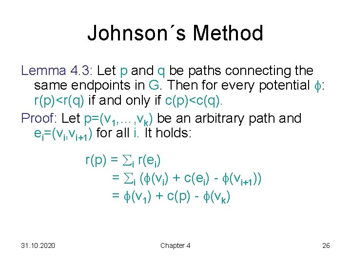
Johnson´s Method Lemma 4. 3: Let p and q be paths connecting the same endpoints in G. Then for every potential : r(p)<r(q) if and only if c(p)<c(q). Proof: Let p=(v 1, …, vk) be an arbitrary path and ei=(vi, vi+1) for all i. It holds: r(p) = i r(ei) = i ( (vi) + c(ei) - (vi+1)) = (v 1) + c(p) - (vk) 31. 10. 2020 Chapter 4 26

Johnson´s Method Lemma 4. 4: Suppose that G has no negative cycles and that all nodes can be reached from s. Let (v)= (s, v) for all v V. With this , r(e)≥ 0 for all e. Proof: • According to our assumption, (s, v) ℝ for all v • We know: for every edge e=(v, w), (s, v)+c(e)≥ (s, w) (otherwise, we have a contradiction to the definition of !) • Therefore, r(e) = (s, v) + c(e) - (s, w) ≥ 0 31. 10. 2020 Chapter 4 27

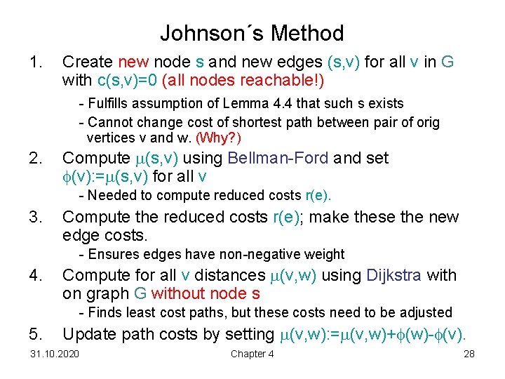
Johnson´s Method 1. Create new node s and new edges (s, v) for all v in G with c(s, v)=0 (all nodes reachable!) - Fulfills assumption of Lemma 4. 4 that such s exists - Cannot change cost of shortest path between pair of orig vertices v and w. (Why? ) 2. Compute (s, v) using Bellman-Ford and set (v): = (s, v) for all v - Needed to compute reduced costs r(e). 3. Compute the reduced costs r(e); make these the new edge costs. - Ensures edges have non-negative weight 4. Compute for all v distances (v, w) using Dijkstra with on graph G without node s - Finds least cost paths, but these costs need to be adjusted 5. Update path costs by setting (v, w): = (v, w)+ (w)- (v). 31. 10. 2020 Chapter 4 28

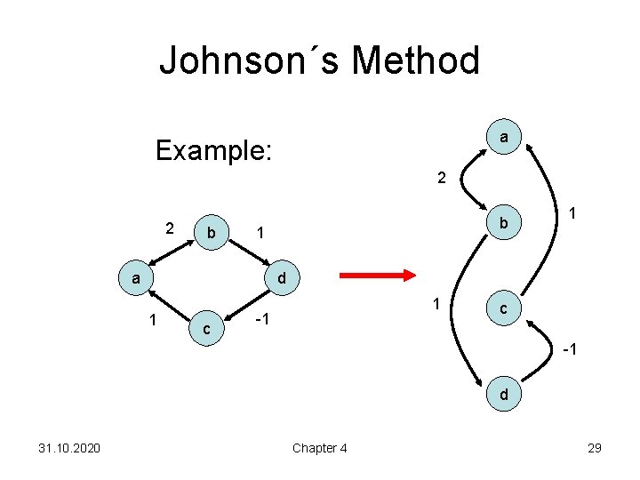
Johnson´s Method a Example: 2 2 b b 1 a 1 d 1 c 1 -1 c -1 d 31. 10. 2020 Chapter 4 29

Johnson´s Method Step 1: create new source s a 2 0 b 0 s 1 0 0 1 c -1 d 31. 10. 2020 Chapter 4 30

Johnson´s Method Step 2: apply Bellman-Ford to s a 2 0 0 s (a)=0 1 b (b)=0 c (c)=-1 0 0 1 -1 d 31. 10. 2020 Chapter 4 (d)=0 31

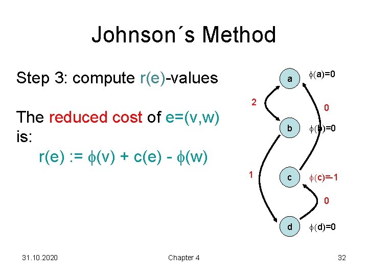
Johnson´s Method Step 3: compute r(e)-values a 2 The reduced cost of e=(v, w) is: r(e) : = (v) + c(e) - (w) 1 (a)=0 0 b (b)=0 c (c)=-1 0 d 31. 10. 2020 Chapter 4 (d)=0 32

Johnson´s Method Step 4: compute all distances (v, w) via Dijkstra a b c d 31. 10. 2020 a 0 1 0 0 b 2 0 2 2 c 3 1 0 0 d 3 1 3 0 Chapter 4 a 2 1 (a)=0 0 b (b)=0 c (c)=-1 0 d (d)=0 33

Johnson´s Method Step 5: compute correct distances via the formula (v, w)= (v, w)+ (w)- (v) a b c d 31. 10. 2020 a 0 1 1 0 b 2 0 3 2 c 2 0 0 -1 d 3 1 4 0 Chapter 4 a 2 1 (a)=0 1 b (b)=0 c (c)=-1 -1 d (d)=0 34

All Pairs Shortest Paths Runtime of Johnson´s Method: O(TBellman-Ford(n, m) + n TDijkstra(n, m)) = O(n m + n(n log n + m)) = O(n m + n 2 log n) when using Fibonacci heaps (amortized runtime). • Problem with the runtime bound: m can be quite large in the worst case (up to ~n 2) • Can we significantly reduce m if we are fine with computing approximate shortest paths? 31. 10. 2020 Chapter 4 35

Question Can we “sparsify” an input graph, i. e. reduce the number of edges, while approximately preserving distances between vertices? If so, the runtime for Johnson’s method can brought down from worst case n 3 : O(n m + n 2 log n) Rest of lecture: How to quickly construct good „graph spanners“. 31. 10. 2020 Chapter 4 36

Graph Spanners Definition 4. 5: Given an undirected graph G=(V, E) with edge costs c: E ℝ, a subgraph H⊆G is an (a, b)-spanner of G iff for all u, v V, d. H(u, v) a d. G(u, v) + b • d. G(u, v): distance of u and v in G • a: multiplicative stretch • b: additive stretch 31. 10. 2020 Chapter 4 37

Graph Spanners Example: all edge costs are 1 G H 31. 10. 2020 Chapter 4 38

Graph Spanners Definition 4. 5: Given an undirected graph G=(V, E) with edge costs c: E ℝ, a subgraph H⊆G is an (a, b) -spanner of G iff for all u, v V, d. H(u, v) a d. G(u, v) + b Observations: 1. Why can we assume WLOG edge costs are nonnegative? (Hint: Problem is trivial in this case. ) 2. Why is this problem not the same as computing a minimum spanning tree? 31. 10. 2020 Chapter 4 39

Graph Spanners Consider the following Greedy algorithm by Althöfer et al. (Discrete Computational Geometry, 1993): E(H): = for each e={u, v} E(G) in the order of non-decreasing edge costs do //if taking e as a shortcut is „a lot“ cheaper than d. H(u, v), then add e if (2 k-1) c(e)<d. H(u, v) then add e to E(H) Q: What is a naive runtime bound on the code above? Theorem 4. 6: For any k 1, |E(H)|=O(n 1+1/k) and the graph H constructed by the Greedy algorithm is a (2 k-1, 0)-spanner. Thorup and Zwick have shown that for any graph G with non-negative edge costs a structure related to H can be built in expected time O(k m n 1/k), which implies that we can then solve the (2 k-1)-approximate APSP in time O(k m n 1/k + n 2+1/k). We will get back to that when we talk about distance oracles. 31. 10. 2020 Chapter 4 40

Graph Spanners Proof of Theorem 4. 6: Lemma 4. 7: H is a (2 k-1, 0)-spanner of G. Proof: • Consider shortest path p from some node a to b in G. • Case 1: If all edges of p exist in H, then d. H(u, v)= d. G(u, v). • Case 2: For any edge {u, v} in p but not in E(H): – Since {u, v} was rejected by the algorithm, d. H(u, v) (2 k-1) c({u, v}). Thus, there is a (u, v)-path P of length at most (2 k-1) c({u, v}) in H. – Replacing edge {u, v} (in G) of p by P (in H) yields the claim. Note: 1. We are implicitly using the fact that in the algorithm, d. H(u, v) is monotonically non-increasing as we loop through edges. (Where do we use this assumption? ) 2. This proof works if 2 k-1 is replaced by any D>=1. 31. 10. 2020 Chapter 4 41

Graph Spanners Consider the following Greedy algorithm by Althöfer et al. (Discrete Computational Geometry, 1993): E(H): = for each e={u, v} E(G) in the order of non-decreasing edge costs do if (2 k-1) c(e)<d. H(u, v) then add e to E(H) Q: What is a naive runtime bound on the code above? Theorem 4. 6: For any k 1, |E(H)|=O(n 1+1/k) and the graph H constructed by the Greedy algorithm is a (2 k-1, 0)-spanner. Left to prove: |E(H)|=O(n 1+1/k) 31. 10. 2020 Chapter 4 42

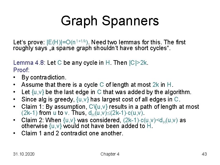
Graph Spanners Let‘s prove: |E(H)|=O(n 1+1/k). Need two lemmas for this. The first roughly says „a sparse graph shouldn‘t have short cycles“. Lemma 4. 8: Let C be any cycle in H. Then |C|>2 k. Proof: • By contradiction. • Assume that there is a cycle C of length at most 2 k in H. • Let {u, v} be the last edge in C that was added by the algorithm. • Since alg is greedy, {u, v} has largest cost of all edges in C. • Claim 1: By assumption, C{u, v} results in a path of length at most (2 k-1) from u to v. Thus, d. H(u, v) (2 k-1) c(u, v). • Claim 2: When {u, v} was considered, (2 k-1) c(u, v)<d. H(u, v) as otherwise {u, v} would not have been added to H. • Claim 1 and 2 contradict one another. 31. 10. 2020 Chapter 4 43

Graph Spanners Let‘s prove: |E(H)|=O(n 1+1/k). Here is the second lemma we need. Lemma 4. 8 implies that H has girth (defined as the minimum cycle length in H) more than 2 k. Lemma 4. 9: Let H be a graph of size n with girth >2 k. Then |E(H)|=O(n 1+1/k). Proof: • If H has at most n+2 n 1+1/k edges, claim is vacuously true. • So assume H is a graph with girth >2 k and at least n+2 n 1+1/k edges. • Repeatedly remove any node from H of degree at most n 1/k and any edges incident to that node, until no such node exists. • The total number of edges removed in this way is at most n (n 1/k+1). (Why? ) • Hence, we obtain a subgraph H´ of H of minimum degree more than n 1/k with at least n 1+1/k edges connecting at most n nodes. • Exercise: show that there cannot be a graph G of size n with girth >2 k and minimum degree more than n 1/k. • Thus, H´ must have a girth of at most 2 k, and therefore also the original graph H. This, however, is a contradiction. 31. 10. 2020 Chapter 4 44

Graph Spanners If we restrict ourselves to unweighted graphs (i. e. , all edges have a cost of 1), we can also construct good additive spanners. Theorem 4. 10: Any n-node graph G has a (1, 2)-spanner with O(n 3/2 log n) edges. Note: Unlike Theorem 4. 6, this result cannot be scaled, i. e. we cannot trade sparsity for approximation precision. Proof: Requires notion of hitting sets! 31. 10. 2020 Chapter 4 45

Hitting Sets Definition 4. 11: Given a collection M of subsets of V, a subset S⊆V is a hitting set of M if it intersects every set in M. Ex. V={1, 2, 3}, M={{1, 2}, {1, 3}, {2, 3}}. What is a min-size hitting set? Is V itself a hitting set? Note: Finding min-size hitting set is NP-complete. Lemma 4. 12: Let M={S 1, …, Sn} be a collection of subsets of V={1, …, n} with |Si| R for all i. There is an algorithm running in O(n. R log n + (n/R)log 2 n) time that finds a hitting set S of M with |S| (n/R)ln n. 31. 10. 2020 Chapter 4 46

Graph Spanners Lemma 4. 12: Let M=(S 1, …, Sn) be a collection of subsets of V={1, …, n} with |Si| R for all i. There is an algorithm running in O(n. R log n + (n/R) log 2 n) time that finds a hitting set S of M with |S| (n/R)ln n. Proof: • Assume w. l. o. g. that |Si|=R for all i. Run the following greedy algorithm: |S|: = //stores the hitting set we are building for each 1 j n, set counter c(j)=|{Si M: j Si}| //number of sets j appears in while M do k: =argmaxj c(j) //which element j appears in largest number of sets? S: =S∪{k} remove any subsets from M containing k and update the counters c(j) accordingly • To obtain the runtime, we store the counts c(j) in a data structure that can support the following operations in O(log n) time: insert an element, return element j with maximum c(j), update key/decrement a given c(j). 31. 10. 2020 Chapter 4 47

Graph Spanners |S|: = for each 1 j n, keep a counter c(j)=|{Si M: j Si}| while M do k: =argmaxj c(j) S: =S∪{k} remove any subsets from M containing k and update the counters c(j) accordingly • total number of inserts: n because of n counters runtime O(n log n) • total number of decrements: n. R because each of the n sets contains just R elements and each of them can only cause one decrement runtime O(n. R log n) • total number of argmax calls: depends on number of iterations of while loop 31. 10. 2020 Chapter 4 48

Graph Spanners Proof of Lemma 4. 12 (continued): • We still need an upper bound on |S| (which gives an upper bound on while loop) • Let mj be the number of sets remaining in M after j passes of the while loop. Then m 0=n. • Let kj be the j-th element added to S, so mj=mj-1–c(kj). • Just before we add kj, the sum of c(j) over all j V{k 1, …, kj-1} must be mj-1 R. Since the algorithm is greedy, c(kj) must be at least the average count, which is mj-1 R/(n-j+1). • Therefore, mj (1 -R/(n-j+1)) mj-1 n Pl=0 j-1 (1 -R/(n-l)) (Hint: Apply bound recursively!) < n (1 -R/n)j n e-Rj/n (using the fact that 1 -x e-x for all x [0, 1]) • Taking j=(n/R) ln n gives mj<1, and therefore mj=0. • Hence, |S| (n/R) ln n. • Thus, the total runtime over all argmax calls is O((n/R)log 2 n). 31. 10. 2020 Chapter 4 49

Graph Spanners • 31. 10. 2020 Chapter 4 50

Graph Spanners • 31. 10. 2020 Chapter 4 51

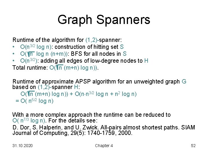
Graph Spanners Runtime of the algorithm for (1, 2)-spanner: • O(n 3/2 log n): construction of hitting set S • O( n log n (n+m)): BFS for all nodes in S • O(n 3/2): adding all edges of low-degree nodes to H Total runtime: O( n (m+n) log n)). Runtime of approximate APSP algorithm for an unweighted graph G based on (1, 2)-spanner H: O( n (m+n) log n)) + O(n n 3/2 log n + n 2 log n) = O( n 5/2 log n) With a more complex approach the runtime can be reduced to O( n 7/3 log n). For the details see: D. Dor, S. Halperin, and U. Zwick. All-pairs almost shortest paths. SIAM Journal of Computing, 29(5): 1740 -1759, 2000. 31. 10. 2020 Chapter 4 52

Graph Spanners Interestingly, the following two results are known: Theorem 4. 13: Any n-node graph G has a (1, 6)-spanner with O(n 4/3) edges. Theorem 4. 14: In general, there is no additive spanner with O(n 4/3 -e) edges for n-node graphs for any e>0. For more info see: Amir Abboud and Greg Bodwin. The 4/3 additive spanner exponent is tight. Proc. of the 48 th ACM Symposium on Theory of Computing (STOC), 2016. 31. 10. 2020 Chapter 4 53

Distance Oracles How to quickly answer distance requests? Naive approach: • Run an APSP algorithm and store all answers in a matrix Problems: • High runtime ( O(nm + n 2 log n) ) • High storage space ( Q(n 2) ) (Why? ) Alternative approach, if approximate answers are sufficient: • Compute additive or multiplicative spanner, and run an APSP algorithm on that spanner. lower runtime • But storage space is still high Better solutions concerning the storage space have been investigated under the concept of distance oracles. 31. 10. 2020 Chapter 4 54

Distance Oracles Definition 4. 15: An a-approximate distance oracle is defined by two algorithms: • a preprocessing algorithm that takes as its input a graph G=(V, E) and returns a summary of G, and • a query algorithm based on the summary of G that takes as its input two vertices u, v V and returns an estimate D(u, v) such that d(u, v) D(u, v) a d(u, v). The quality of an a-approximate distance oracle is defined by its query time q(n), preprocessing time p(m, n), and storage space s(n). The goal is to minimize all of these quantities. Thorup and Zwick (STOC 2001) have shown the following result for graphs of non-negative edge costs: Theorem 4. 16: For all k 1 there exists a (2 k-1)-approximate distance oracle using O(k n 1+1/k) space and O(m n 1/k) time for preprocessing that can answer queries in O(k) time (where we hide logarithmic factors in the O-notation). 31. 10. 2020 Chapter 4 55

Distance Oracles Theorem 4. 16: For all k 1 there exists a (2 k-1)-approximate distance oracle using O(k n 1+1/k) space and O(m n 1/k) time for preprocessing that can answer queries in O(k) time (where we hide logarithmic factors in the O-notation). Proof: k=1: trivial. Just run our APSP algorithm. k=2: Consider the following preprocessing algorithm: A: = random subset S⊆V of size O( n log n) for each a A run Dijkstra to compute d(a, v) for all v V for each v VA do p. A(v): =argminy A d(v, y) //find vertex in A closest to v // find vertices in V closer to v than those in A run Dijkstra to compute A(v): ={x V | d(v, x)<d(v, p. A(v))} B(v): =A∪A(v) store p. A(v) under v for all x B(v), store d(v, x) under key (v, x) in a hash table • It is easy to show that with high probability A is a hitting set of M={ N n (v) | v V}, where N n (v) is the set containing the closest n nodes to v. 31. 10. 2020 Chapter 4 56

Distance Oracles A helpful lemma to bound storage requirements: Lemma 4. 17: |B(v)| O( n log n). Proof: • It suffices to show that |A(v)| n since by construction |A|=O( n log n). • Because A hits the closest n nodes to v with high probability, some node a A is also in N n (v). • Thus, all nodes closer to v than a are also in N n (v). • By the definition of A(v), this implies that A(v) ⊆ N n (v) , and therefore, |A(v)| n. 31. 10. 2020 Chapter 4 57

Distance Oracles Proof of Theorem 4. 16 (continued): Now we can bound the quality of the distance oracle. Storage • Lemma 4. 17 implies that the storage space needed by our distance oracle is O(n n log n). Query time • A query (u, v) is processed as follows: if d(u, v) is stored in the hash table then return d(u, v) =: D(u, v) else return d(u, p. A(u))+d(v, p. A(u)) =: D(u, v) • This obviously takes constant time. Query accuracy/quality For current case k=2, need to show that d(u, v) D(u, v) 3 d(u, v). 31. 10. 2020 Chapter 4 58

Distance Oracles Claim: d(u, v) D(u, v) 3 d(u, v). • Suppose that v B(u), as otherwise D(u, v)=d(u, v). • By the triangle inequality we have d(u, v) d(u, p. A(u))+d(v, p. A(u)) = D(u, v) • In order to show that D(u, v) 3 d(u, v), we use the triangle inequality again to obtain D(u, v) = d(u, p. A(u))+d(p. A(u), v) d(u, p. A(u))+(d(p. A(u), u)+d(u, v)) = 2 d(u, p. A(u)) + d(u, v) 3 d(u, v) (Why? ) 31. 10. 2020 Chapter 4 59

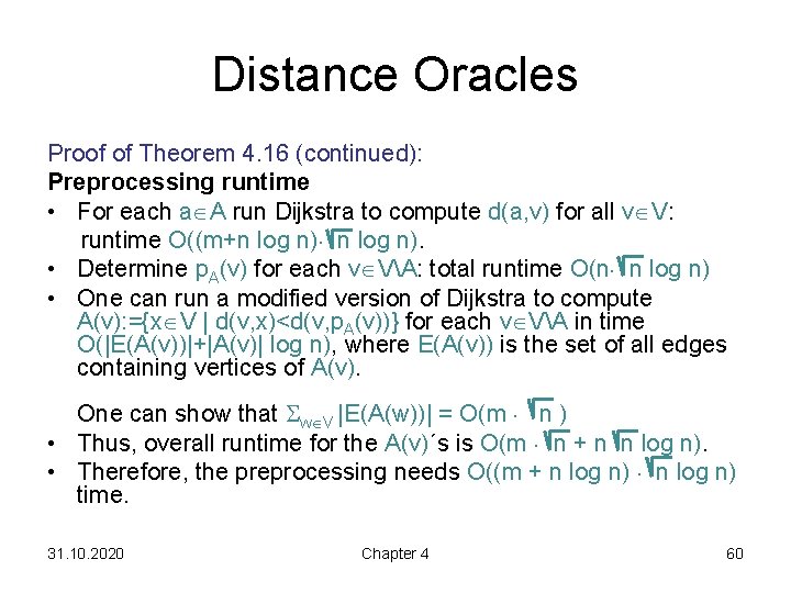
Distance Oracles Proof of Theorem 4. 16 (continued): Preprocessing runtime • For each a A run Dijkstra to compute d(a, v) for all v V: runtime O((m+n log n) n log n). • Determine p. A(v) for each v VA: total runtime O(n n log n) • One can run a modified version of Dijkstra to compute A(v): ={x V | d(v, x)<d(v, p. A(v))} for each v VA in time O(|E(A(v))|+|A(v)| log n), where E(A(v)) is the set of all edges containing vertices of A(v). One can show that Sw V |E(A(w))| = O(m n ) • Thus, overall runtime for the A(v)´s is O(m n + n n log n). • Therefore, the preprocessing needs O((m + n log n) time. 31. 10. 2020 Chapter 4 60

Distance Oracles Proof of Theorem 4. 16 (continued): The algorithm for general k proceeds by taking many related samples A 0, …, Ak instead of just a single sample A. Concretely, it does the following: • Let A 0=V and Ak=. For each 1 i k-1, choose a random Ai⊆Ai-1 of size (|Ai-1|/n 1/k) log n = O(n 1 -i/k log n). • Let pi(v) be the closest node to v in Ai. If d(v, pi(v))=d(v, pi+1(v)) then let pi(v)=pi+1(v). • For all v V and i<k-1, define Ai(v) = { x Ai | d(v, x) < d(v, pi+1(v)) } B(v) = Ak-1∪(Ui=0 k-2 Ai(v)) • For all v V and all x B(v), store d(v, x) in a hash table. Also store for each v V and each i k-1, pi(v). A query for (u, v) then works as follows: w: =p 0=v for i=1 to k do if w B(u) then return d(u, w)+d(w, v) else w: =pi(u) ; swap u and v For more information see: Mikkel Thorup and Uri Zwick. Approximate distance oracles. In Proc. of the 33 rd ACM Symposium on Theory of Computing (STOC), 2001. 31. 10. 2020 Chapter 4 61

Next Chapter Matching algorithms… 31. 10. 2020 Chapter 4 62