Fundamental Accounting Principles Twenty Third Edition Chapter 23

Fundamental Accounting Principles Twenty Third Edition Chapter 23 Flexible Budgets and Standard Costs © Mc. Graw-Hill Education. All rights reserved. Authorized only for instructor use in the classroom. No reproduction or further distribution permitted without the prior written consent of Mc. Graw-Hill Education.

5 - 2 Learning Objectives (1 of 2) CONCEPTUAL C 1 Define standard costs and explain how standard cost information is useful for management by exception. C 2 Describe cost variances and what they reveal about performance. ANALYTICAL A 1 Analyze changes in sales from expected amounts. © Mc. Graw-Hill Education. 23 -2

5 - 3 Learning Objectives (2 of 2) PROCEDURAL P 1 Prepare a flexible budget and interpret a flexible budget performance report. P 2 Compute materials and labor variances. P 3 Compute overhead spending and efficiency variances. P 4 Compute overhead spending and efficiency variances. (Appendix 23 A) P 5 Prepare journal entries for standard costs and account for price and quantity variances. (Appendix 23 A) © Mc. Graw-Hill Education. 23 -3

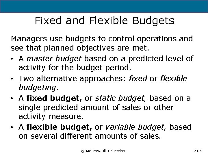
5 - 4 Fixed and Flexible Budgets Managers use budgets to control operations and see that planned objectives are met. • A master budget based on a predicted level of activity for the budget period. • Two alternative approaches: fixed or flexible budgeting. • A fixed budget, or static budget, based on a single predicted amount of sales or other activity measure. • A flexible budget, or variable budget, based on several different amounts of sales. © Mc. Graw-Hill Education. 23 -4

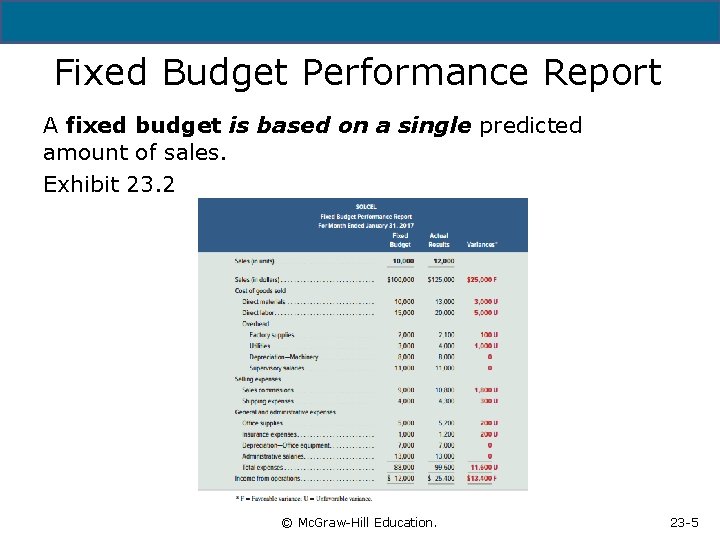
Fixed Budget Performance Report A fixed budget is based on a single predicted amount of sales. Exhibit 23. 2 Copyright © 201 Mc. Graw-Hill Education. All rights reserved. No reproduction or distribution. Education. without the prior written consent of Mc. Graw-Hill © Mc. Graw-Hill Education. 23 -5

5 - 6 Purpose of Flexible Budgets • Flexible Budgets – Show revenues and expenses that should have occurred at the actual level of activity. – May be prepared for several activity levels in the relevant range. – Reveal variances due to good cost control or lack of cost control. – Improve performance evaluation and helps managers focus on problem areas. © Mc. Graw-Hill Education. 23 -6

5 - 7 Learning Objective P 1: Prepare a flexible budget and interpret a flexible budget performance report. © Mc. Graw-Hill Education. 23 -7

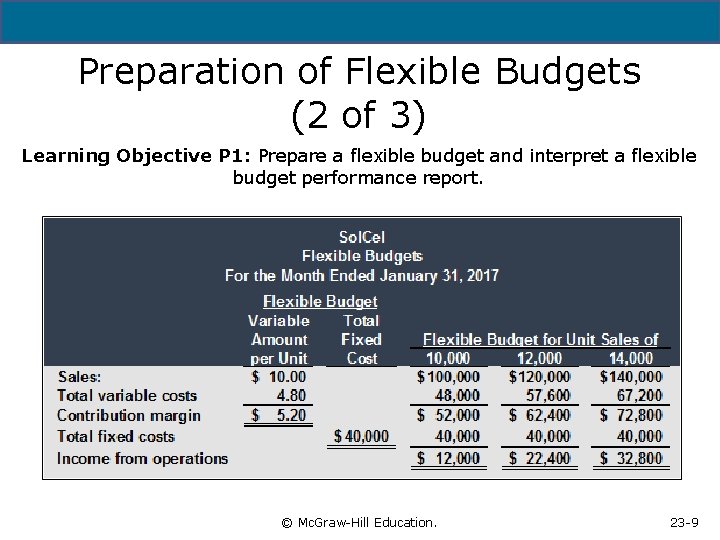
5 - 8 Preparation of Flexible Budgets (1 of 3) Learning Objective P 1: Prepare a flexible budget and interpret a flexible budget performance report. • To flex a budget for different activity levels, we must know how costs behave with changes in activity levels. – Total variable costs change in direct proportion to changes in activity. – Total fixed costs remain unchanged within the relevant range. © Mc. Graw-Hill Education. 23 -8

Preparation of Flexible Budgets (2 of 3) Learning Objective P 1: Prepare a flexible budget and interpret a flexible budget performance report. Copyright © 201 Mc. Graw-Hill Education. All rights reserved. No reproduction or distribution. Education. without the prior written consent of Mc. Graw-Hill © Mc. Graw-Hill Education. 23 -9

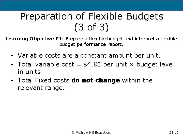
5 - 10 Preparation of Flexible Budgets (3 of 3) Learning Objective P 1: Prepare a flexible budget and interpret a flexible budget performance report. • Variable costs are a constant amount per unit. • Total variable cost = $4. 80 per unit × budget level in units • Total Fixed costs do not change within the relevant range. © Mc. Graw-Hill Education. 23 -10

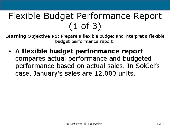
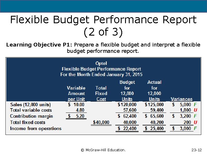
5 - 11 Flexible Budget Performance Report (1 of 3) Learning Objective P 1: Prepare a flexible budget and interpret a flexible budget performance report. • A flexible budget performance report compares actual performance and budgeted performance based on actual sales. In Sol. Cel’s case, January’s sales are 12, 000 units. © Mc. Graw-Hill Education. 23 -11

Flexible Budget Performance Report (2 of 3) Learning Objective P 1: Prepare a flexible budget and interpret a flexible budget performance report. Copyright © 201 Mc. Graw-Hill Education. All rights reserved. No reproduction or distribution. Education. without the prior written consent of Mc. Graw-Hill © Mc. Graw-Hill Education. 23 -12

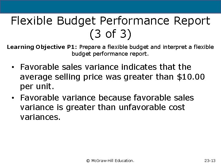
5 - 13 Flexible Budget Performance Report (3 of 3) Learning Objective P 1: Prepare a flexible budget and interpret a flexible budget performance report. • Favorable sales variance indicates that the average selling price was greater than $10. 00 per unit. • Favorable variance because favorable sales variance is greater than unfavorable cost variances. © Mc. Graw-Hill Education. 23 -13

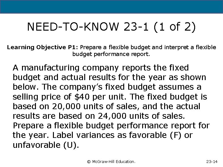
5 - 14 NEED-TO-KNOW 23 -1 (1 of 2) Learning Objective P 1: Prepare a flexible budget and interpret a flexible budget performance report. A manufacturing company reports the fixed budget and actual results for the year as shown below. The company’s fixed budget assumes a selling price of $40 per unit. The fixed budget is based on 20, 000 units of sales, and the actual results are based on 24, 000 units of sales. Prepare a flexible budget performance report for the year. Label variances as favorable (F) or unfavorable (U). © Mc. Graw-Hill Education. 23 -14

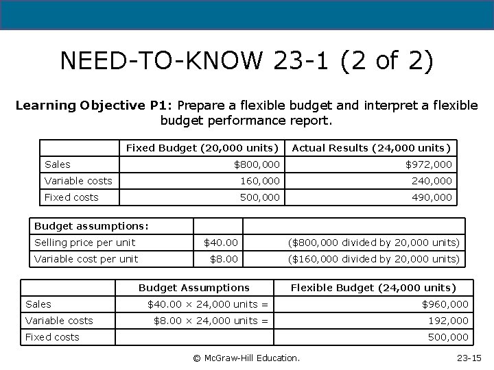
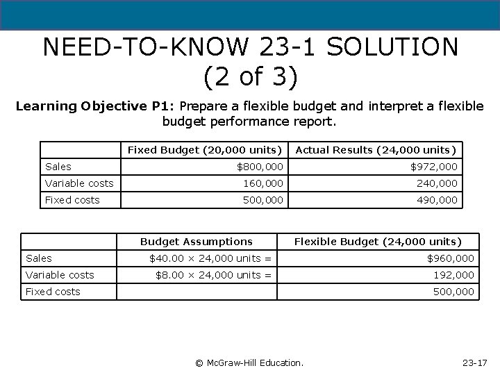
NEED-TO-KNOW 23 -1 (2 of 2) Learning Objective P 1: Prepare a flexible budget and interpret a flexible budget performance report. Fixed Budget (20, 000 units) Actual Results (24, 000 units) $800, 000 $972, 000 Variable costs 160, 000 240, 000 Fixed costs 500, 000 490, 000 Sales Budget assumptions: Selling price per unit Variable cost per unit $40. 00 ($800, 000 divided by 20, 000 units) $8. 00 ($160, 000 divided by 20, 000 units) Budget Assumptions Sales Variable costs Flexible Budget (24, 000 units) $40. 00 × 24, 000 units = $960, 000 $8. 00 × 24, 000 units = 192, 000 Fixed costs Copyright © 201 Mc. Graw-Hill Education. All rights reserved. No reproduction or distribution. Education. without the prior written consent of Mc. Graw-Hill © Mc. Graw-Hill Education. 500, 000 23 -15

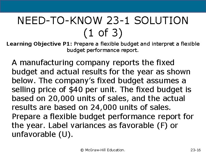
5 - 16 NEED-TO-KNOW 23 -1 SOLUTION (1 of 3) Learning Objective P 1: Prepare a flexible budget and interpret a flexible budget performance report. A manufacturing company reports the fixed budget and actual results for the year as shown below. The company’s fixed budget assumes a selling price of $40 per unit. The fixed budget is based on 20, 000 units of sales, and the actual results are based on 24, 000 units of sales. Prepare a flexible budget performance report for the year. Label variances as favorable (F) or unfavorable (U). © Mc. Graw-Hill Education. 23 -16

NEED-TO-KNOW 23 -1 SOLUTION (2 of 3) Learning Objective P 1: Prepare a flexible budget and interpret a flexible budget performance report. Fixed Budget (20, 000 units) Actual Results (24, 000 units) $800, 000 $972, 000 Variable costs 160, 000 240, 000 Fixed costs 500, 000 490, 000 Sales Budget Assumptions Sales Variable costs Flexible Budget (24, 000 units) $40. 00 × 24, 000 units = $960, 000 $8. 00 × 24, 000 units = 192, 000 Fixed costs Copyright © 201 Mc. Graw-Hill Education. All rights reserved. No reproduction or distribution. Education. without the prior written consent of Mc. Graw-Hill © Mc. Graw-Hill Education. 500, 000 23 -17

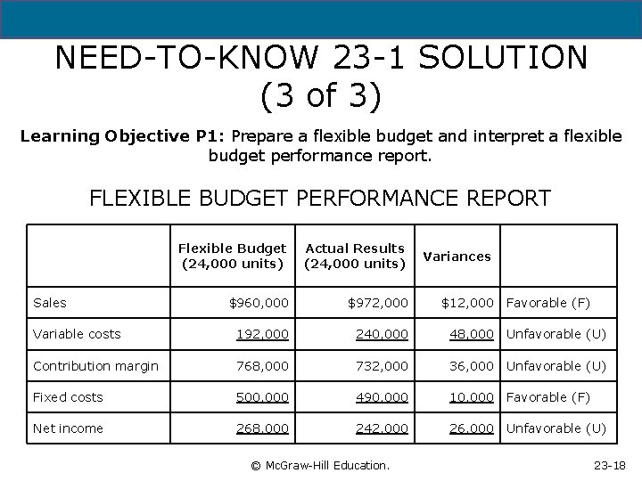
NEED-TO-KNOW 23 -1 SOLUTION (3 of 3) Learning Objective P 1: Prepare a flexible budget and interpret a flexible budget performance report. FLEXIBLE BUDGET PERFORMANCE REPORT Flexible Budget (24, 000 units) Actual Results (24, 000 units) Variances $960, 000 $972, 000 $12, 000 Variable costs 192, 000 240, 000 48, 000 Unfavorable (U) Contribution margin 768, 000 732, 000 36, 000 Unfavorable (U) Fixed costs 500, 000 490, 000 10, 000 Favorable (F) Net income 268, 000 242, 000 26, 000 Unfavorable (U) Sales Favorable (F) Copyright © 201 Mc. Graw-Hill Education. All rights reserved. No reproduction or distribution. Education. without the prior written consent of Mc. Graw-Hill © Mc. Graw-Hill Education. 23 -18

5 - 19 Learning Objective C 1: Define standard costs and explain how standard cost information is useful for management by exception. © Mc. Graw-Hill Education. 23 -19

5 - 20 Standard Costs Learning Objective C 1: Define standard costs and explain how standard cost information is useful for management by exception. Standard costs can be used in a flexible budgeting system to enable management to better understand the reasons for variances • Standard costs are – Based on carefully predetermined amounts. – Used for planning materials, labor, and overhead requirements. – The expected level of performance. – Benchmarks for measuring performance. © Mc. Graw-Hill Education. 23 -20

5 - 21 Identifying Standard Costs Learning Objective C 1: Define standard costs and explain how standard cost information is useful for management by exception. • Managerial accountants, engineers, personnel administrators, and other managers combine their efforts to set standard costs. • Standards should be challenging but attainable, and should acknowledge machine breakdowns, material waste, and idle time. • Engineer • Production Manager • Human Resources Manager • Managerial Accountant © Mc. Graw-Hill Education. 23 -21

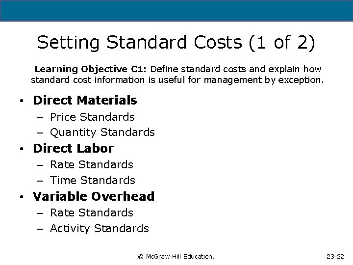
5 - 22 Setting Standard Costs (1 of 2) Learning Objective C 1: Define standard costs and explain how standard cost information is useful for management by exception. • Direct Materials – Price Standards – Quantity Standards • Direct Labor – Rate Standards – Time Standards • Variable Overhead – Rate Standards – Activity Standards © Mc. Graw-Hill Education. 23 -22

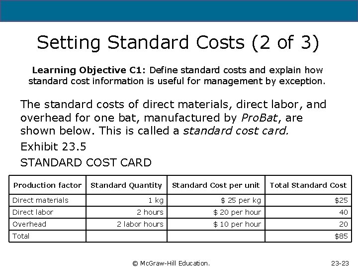
Setting Standard Costs (2 of 3) Learning Objective C 1: Define standard costs and explain how standard cost information is useful for management by exception. The standard costs of direct materials, direct labor, and overhead for one bat, manufactured by Pro. Bat, are shown below. This is called a standard cost card. Exhibit 23. 5 STANDARD COST CARD Production factor Direct materials Direct labor Overhead Standard Quantity Standard Cost per unit Total Standard Cost 1 kg $ 25 per kg $25 2 hours $ 20 per hour 40 2 labor hours $ 10 per hour 20 Total Copyright © 201 Mc. Graw-Hill Education. All rights reserved. No reproduction or distribution without the prior written consent of Mc. Graw-Hill © Mc. Graw-Hill Education. $85 23 -23

5 - 24 Setting Standard Costs (3 of 3) Learning Objective C 1: Define standard costs and explain how standard cost information is useful for management by exception. These standard cost amounts are then used to prepare manufacturing budgets for a budgeted level of production. © Mc. Graw-Hill Education. 23 -24

5 - 25 Learning Objective C 2: Describe cost variances and what they reveal about performance. © Mc. Graw-Hill Education. 23 -25

5 - 26 Cost Variances Learning Objective C 2: Describe cost variances and what they reveal about performance. • Cost variance difference between actual and standard cost. • if actual cost > standard cost Variance is unfavorable (U). • If actual cost < standard cost Variance is favorable (F). © Mc. Graw-Hill Education. 23 -26

5 - 27 Cost Variance Analysis (1 of 2) Learning Objective C 2: Describe cost variances and what they reveal about performance. • Prepare Reports Analyze Variances Questions and Answers Take Action • The process is repeated again. • Variance analysis involves preparing a standard cost performance report and comparing actual costs with standard costs. • We then investigate variances by asking for explanations and possible causes for the variances. © Mc. Graw-Hill Education. 23 -27

5 - 28 Cost Variance Analysis (2 of 2) Learning Objective C 2: Describe cost variances and what they reveal about performance. • We should correct problems that caused unfavorable variances and possibly adopt and reward the practices that resulted in favorable variances. © Mc. Graw-Hill Education. 23 -28

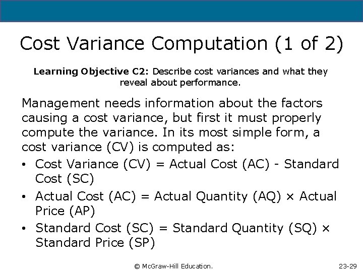
5 - 29 Cost Variance Computation (1 of 2) Learning Objective C 2: Describe cost variances and what they reveal about performance. Management needs information about the factors causing a cost variance, but first it must properly compute the variance. In its most simple form, a cost variance (CV) is computed as: • Cost Variance (CV) = Actual Cost (AC) - Standard Cost (SC) • Actual Cost (AC) = Actual Quantity (AQ) × Actual Price (AP) • Standard Cost (SC) = Standard Quantity (SQ) × Standard Price (SP) © Mc. Graw-Hill Education. 23 -29

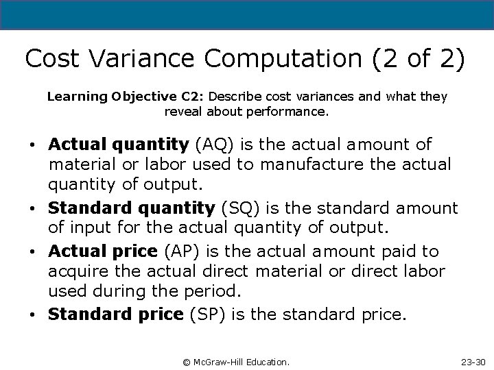
5 - 30 Cost Variance Computation (2 of 2) Learning Objective C 2: Describe cost variances and what they reveal about performance. • Actual quantity (AQ) is the actual amount of material or labor used to manufacture the actual quantity of output. • Standard quantity (SQ) is the standard amount of input for the actual quantity of output. • Actual price (AP) is the actual amount paid to acquire the actual direct material or direct labor used during the period. • Standard price (SP) is the standard price. © Mc. Graw-Hill Education. 23 -30

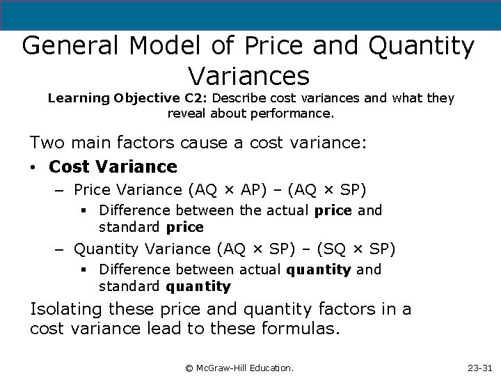
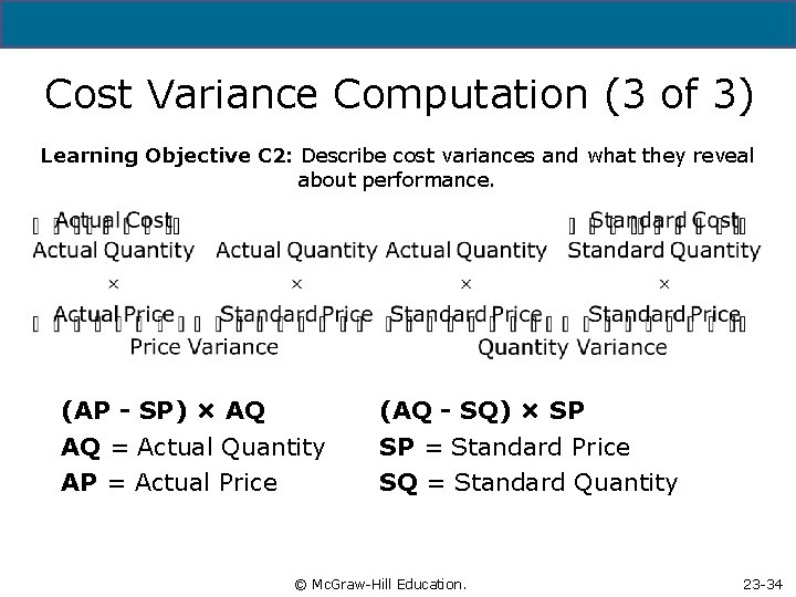
5 - 31 General Model of Price and Quantity Variances Learning Objective C 2: Describe cost variances and what they reveal about performance. Two main factors cause a cost variance: • Cost Variance – Price Variance (AQ × AP) – (AQ × SP) § Difference between the actual price and standard price – Quantity Variance (AQ × SP) – (SQ × SP) § Difference between actual quantity and standard quantity Isolating these price and quantity factors in a cost variance lead to these formulas. © Mc. Graw-Hill Education. 23 -31

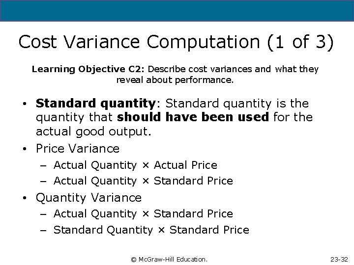
5 - 32 Cost Variance Computation (1 of 3) Learning Objective C 2: Describe cost variances and what they reveal about performance. • Standard quantity: Standard quantity is the quantity that should have been used for the actual good output. • Price Variance – Actual Quantity × Actual Price – Actual Quantity × Standard Price • Quantity Variance – Actual Quantity × Standard Price – Standard Quantity × Standard Price © Mc. Graw-Hill Education. 23 -32

5 - 33 Cost Variance Computation (2 of 3) Learning Objective C 2: Describe cost variances and what they reveal about performance. • Standard Price: Standard price is the amount that should have been paid for the resources acquired. © Mc. Graw-Hill Education. 23 -33

5 - 34 Cost Variance Computation (3 of 3) Learning Objective C 2: Describe cost variances and what they reveal about performance. (AP - SP) × AQ AQ = Actual Quantity AP = Actual Price (AQ - SQ) × SP SP = Standard Price SQ = Standard Quantity © Mc. Graw-Hill Education. 23 -34

5 - 35 Learning Objective P 2: Compute materials and labor variances. © Mc. Graw-Hill Education. 23 -35

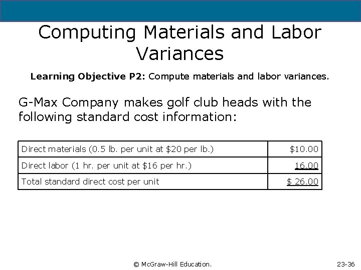
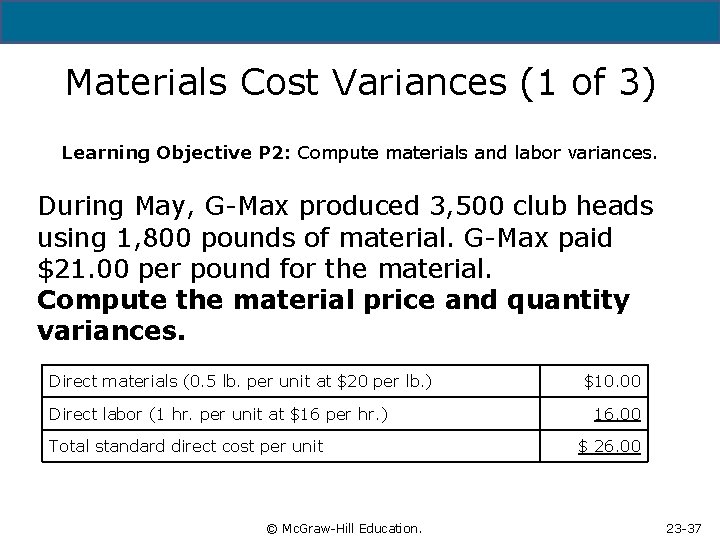
5 - 36 Computing Materials and Labor Variances Learning Objective P 2: Compute materials and labor variances. G-Max Company makes golf club heads with the following standard cost information: Direct materials (0. 5 lb. per unit at $20 per lb. ) Direct labor (1 hr. per unit at $16 per hr. ) Total standard direct cost per unit © Mc. Graw-Hill Education. $10. 00 16. 00 $ 26. 00 23 -36

Materials Cost Variances (1 of 3) Learning Objective P 2: Compute materials and labor variances. During May, G-Max produced 3, 500 club heads using 1, 800 pounds of material. G-Max paid $21. 00 per pound for the material. Compute the material price and quantity variances. Direct materials (0. 5 lb. per unit at $20 per lb. ) Direct labor (1 hr. per unit at $16 per hr. ) Total standard direct cost per unit Copyright © 201 Mc. Graw-Hill Education. All rights reserved. No reproduction or distribution without the prior written consent of Mc. Graw-Hill © Mc. Graw-Hill Education. $10. 00 16. 00 $ 26. 00 23 -37

Materials Cost Variances (2 of 3) Learning Objective P 2: Compute materials and labor variances. Use this information to compute the material price and quantity variances before you go to the next slide. Copyright © 201 Mc. Graw-Hill Education. All rights reserved. No reproduction or distribution without the prior written consent of Mc. Graw-Hill © Mc. Graw-Hill Education. 23 -38

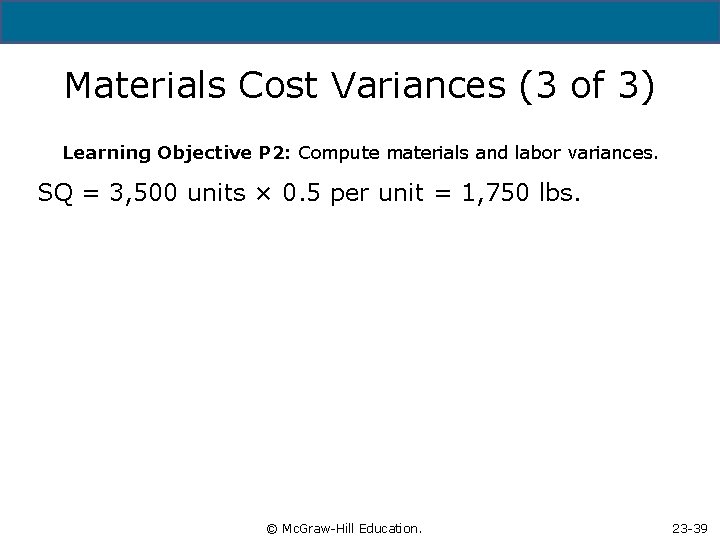
5 - 39 Materials Cost Variances (3 of 3) Learning Objective P 2: Compute materials and labor variances. SQ = 3, 500 units × 0. 5 per unit = 1, 750 lbs. © Mc. Graw-Hill Education. 23 -39

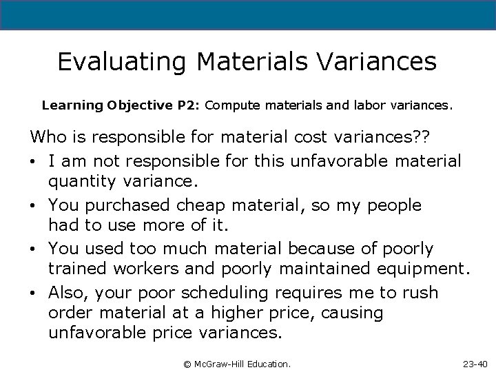
5 - 40 Evaluating Materials Variances Learning Objective P 2: Compute materials and labor variances. Who is responsible for material cost variances? ? • I am not responsible for this unfavorable material quantity variance. • You purchased cheap material, so my people had to use more of it. • You used too much material because of poorly trained workers and poorly maintained equipment. • Also, your poor scheduling requires me to rush order material at a higher price, causing unfavorable price variances. © Mc. Graw-Hill Education. 23 -40

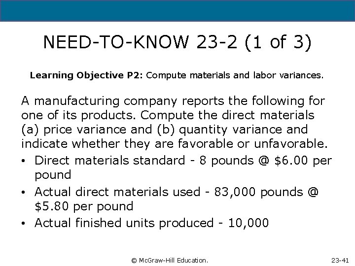
5 - 41 NEED-TO-KNOW 23 -2 (1 of 3) Learning Objective P 2: Compute materials and labor variances. A manufacturing company reports the following for one of its products. Compute the direct materials (a) price variance and (b) quantity variance and indicate whether they are favorable or unfavorable. • Direct materials standard - 8 pounds @ $6. 00 per pound • Actual direct materials used - 83, 000 pounds @ $5. 80 per pound • Actual finished units produced - 10, 000 © Mc. Graw-Hill Education. 23 -41

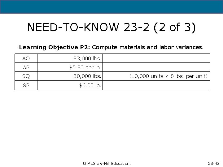
5 - 42 NEED-TO-KNOW 23 -2 (2 of 3) Learning Objective P 2: Compute materials and labor variances. AQ 83, 000 lbs. AP $5. 80 per lb. SQ 80, 000 lbs. SP $6. 00 lb. (10, 000 units × 8 lbs. per unit) © Mc. Graw-Hill Education. 23 -42

5 - 43 NEED-TO-KNOW 23 -2 (3 of 3) Learning Objective P 2: Compute materials and labor variances. © Mc. Graw-Hill Education. 23 -43

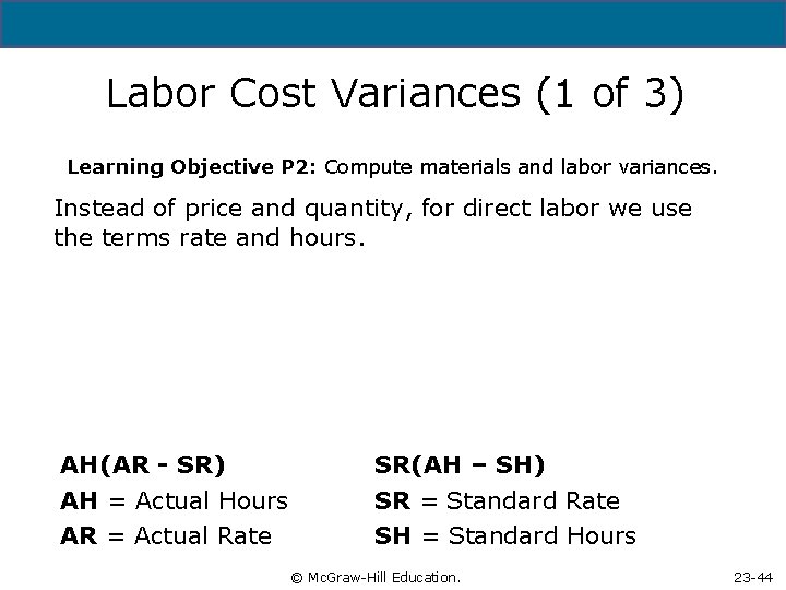
5 - 44 Labor Cost Variances (1 of 3) Learning Objective P 2: Compute materials and labor variances. Instead of price and quantity, for direct labor we use the terms rate and hours. AH(AR - SR) AH = Actual Hours AR = Actual Rate SR(AH – SH) SR = Standard Rate SH = Standard Hours © Mc. Graw-Hill Education. 23 -44

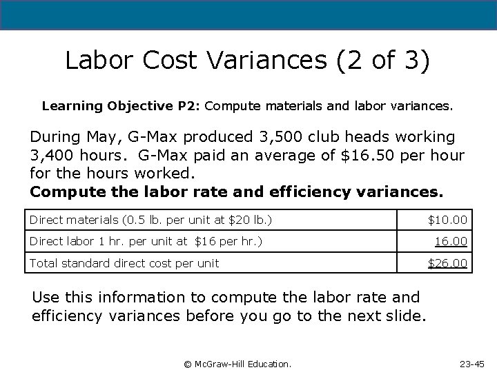
Labor Cost Variances (2 of 3) Learning Objective P 2: Compute materials and labor variances. During May, G-Max produced 3, 500 club heads working 3, 400 hours. G-Max paid an average of $16. 50 per hour for the hours worked. Compute the labor rate and efficiency variances. Direct materials (0. 5 lb. per unit at $20 lb. ) Direct labor 1 hr. per unit at $16 per hr. ) Total standard direct cost per unit $10. 00 16. 00 $26. 00 Use this information to compute the labor rate and efficiency variances before you go to the next slide. Copyright © 201 Mc. Graw-Hill Education. All rights reserved. No reproduction or distribution without the prior written consent of Mc. Graw-Hill © Mc. Graw-Hill Education. 23 -45

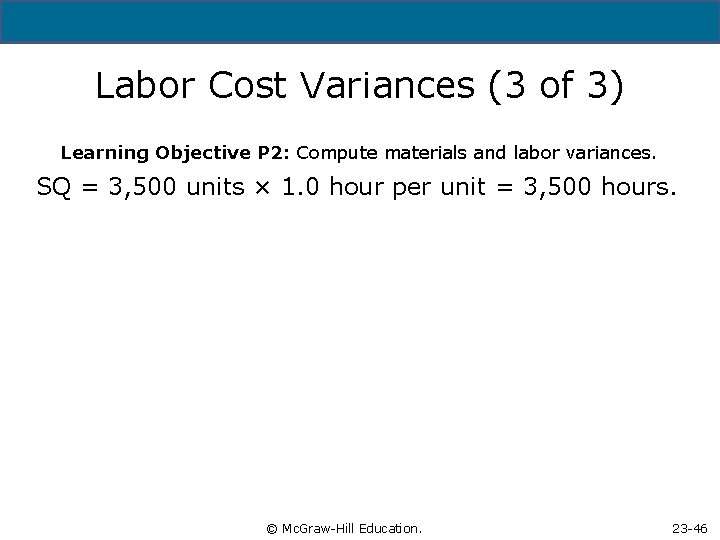
5 - 46 Labor Cost Variances (3 of 3) Learning Objective P 2: Compute materials and labor variances. SQ = 3, 500 units × 1. 0 hour per unit = 3, 500 hours. © Mc. Graw-Hill Education. 23 -46

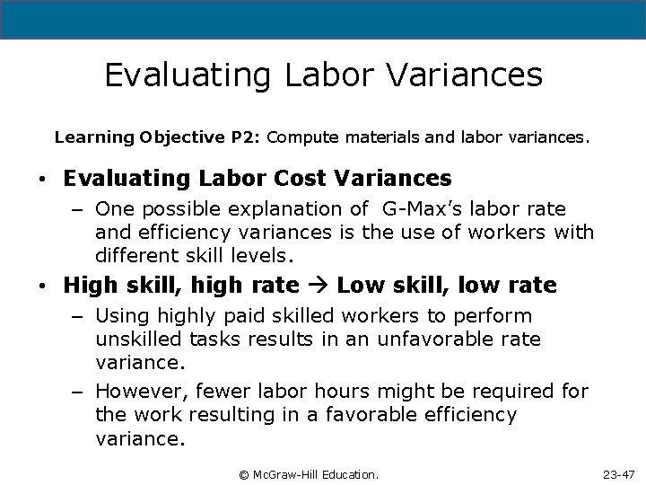
5 - 47 Evaluating Labor Variances Learning Objective P 2: Compute materials and labor variances. • Evaluating Labor Cost Variances – One possible explanation of G-Max’s labor rate and efficiency variances is the use of workers with different skill levels. • High skill, high rate Low skill, low rate – Using highly paid skilled workers to perform unskilled tasks results in an unfavorable rate variance. – However, fewer labor hours might be required for the work resulting in a favorable efficiency variance. © Mc. Graw-Hill Education. 23 -47

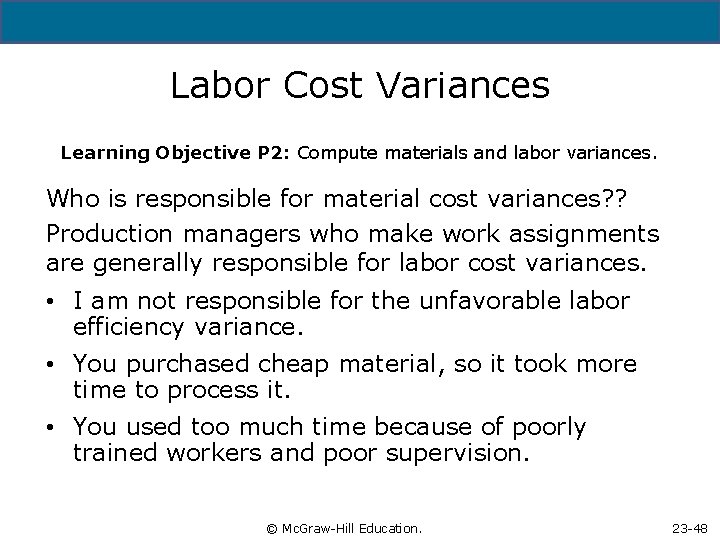
5 - 48 Labor Cost Variances Learning Objective P 2: Compute materials and labor variances. Who is responsible for material cost variances? ? Production managers who make work assignments are generally responsible for labor cost variances. • I am not responsible for the unfavorable labor efficiency variance. • You purchased cheap material, so it took more time to process it. • You used too much time because of poorly trained workers and poor supervision. © Mc. Graw-Hill Education. 23 -48

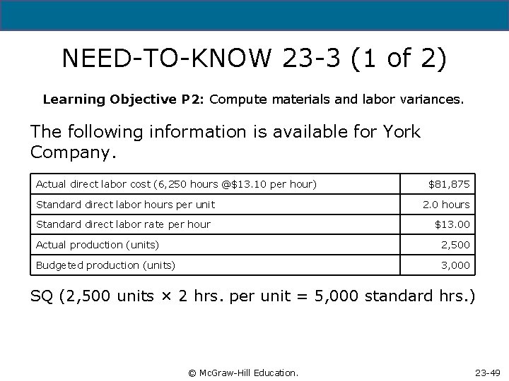
5 - 49 NEED-TO-KNOW 23 -3 (1 of 2) Learning Objective P 2: Compute materials and labor variances. The following information is available for York Company. Actual direct labor cost (6, 250 hours @$13. 10 per hour) Standard direct labor hours per unit Standard direct labor rate per hour $81, 875 2. 0 hours $13. 00 Actual production (units) 2, 500 Budgeted production (units) 3, 000 SQ (2, 500 units × 2 hrs. per unit = 5, 000 standard hrs. ) © Mc. Graw-Hill Education. 23 -49

NEED-TO-KNOW 23 -3 (2 of 2) Learning Objective P 2: Compute materials and labor variances. *SQ: (2, 500 units × 2 hrs. per unit = 5, 000 standard hrs. ) Copyright © 201 Mc. Graw-Hill Education. All rights reserved. No reproduction or distribution without the prior written consent of Mc. Graw-Hill © Mc. Graw-Hill Education. 23 -50

5 - 51 Learning Objective P 3: Compute overhead spending and efficiency variances. © Mc. Graw-Hill Education. 23 -51

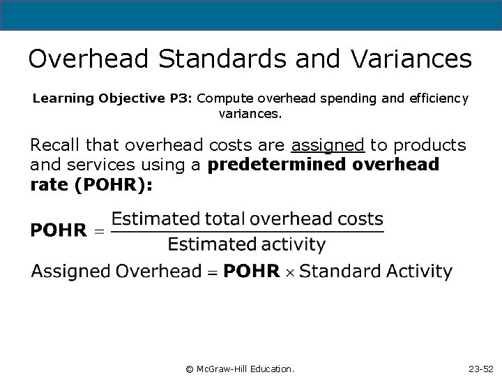
5 - 52 Overhead Standards and Variances Learning Objective P 3: Compute overhead spending and efficiency variances. Recall that overhead costs are assigned to products and services using a predetermined overhead rate (POHR): © Mc. Graw-Hill Education. 23 -52

5 - 53 Standard Overhead Rate (1 of 2) Learning Objective P 3: Compute overhead spending and efficiency variances. • Standard overhead costs are the overhead amounts expected to occur at a certain activity level. • To allocate overhead costs to products or services, management needs to establish the standard overhead cost rate. Uses a threestep process: © Mc. Graw-Hill Education. 23 -53

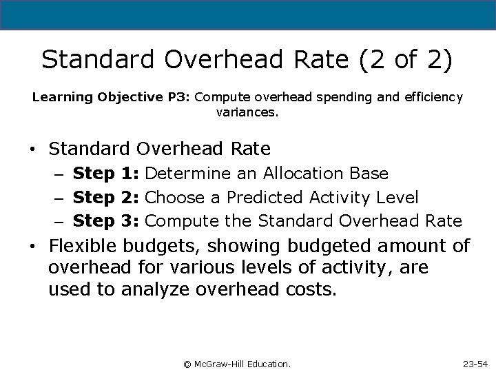
5 - 54 Standard Overhead Rate (2 of 2) Learning Objective P 3: Compute overhead spending and efficiency variances. • Standard Overhead Rate – Step 1: Determine an Allocation Base – Step 2: Choose a Predicted Activity Level – Step 3: Compute the Standard Overhead Rate • Flexible budgets, showing budgeted amount of overhead for various levels of activity, are used to analyze overhead costs. © Mc. Graw-Hill Education. 23 -54

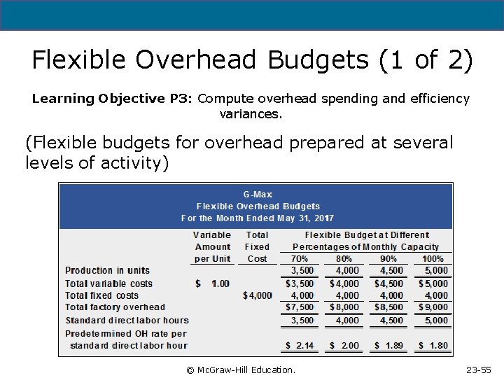
Flexible Overhead Budgets (1 of 2) Learning Objective P 3: Compute overhead spending and efficiency variances. (Flexible budgets for overhead prepared at several levels of activity) Copyright © 201 Mc. Graw-Hill Education. All rights reserved. No reproduction or distribution without the prior written consent of Mc. Graw-Hill © Mc. Graw-Hill Education. 23 -55

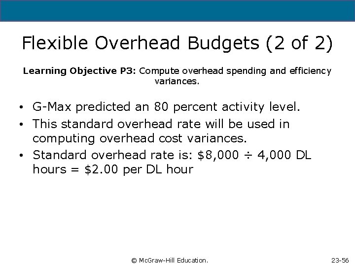
5 - 56 Flexible Overhead Budgets (2 of 2) Learning Objective P 3: Compute overhead spending and efficiency variances. • G-Max predicted an 80 percent activity level. • This standard overhead rate will be used in computing overhead cost variances. • Standard overhead rate is: $8, 000 ÷ 4, 000 DL hours = $2. 00 per DL hour © Mc. Graw-Hill Education. 23 -56

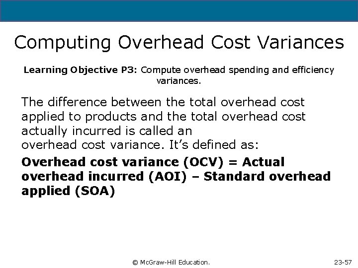
5 - 57 Computing Overhead Cost Variances Learning Objective P 3: Compute overhead spending and efficiency variances. The difference between the total overhead cost applied to products and the total overhead cost actually incurred is called an overhead cost variance. It’s defined as: Overhead cost variance (OCV) = Actual overhead incurred (AOI) – Standard overhead applied (SOA) © Mc. Graw-Hill Education. 23 -57

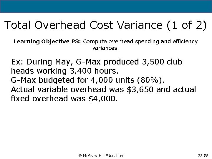
5 - 58 Total Overhead Cost Variance (1 of 2) Learning Objective P 3: Compute overhead spending and efficiency variances. Ex: During May, G-Max produced 3, 500 club heads working 3, 400 hours. G-Max budgeted for 4, 000 units (80%). Actual variable overhead was $3, 650 and actual fixed overhead was $4, 000. © Mc. Graw-Hill Education. 23 -58

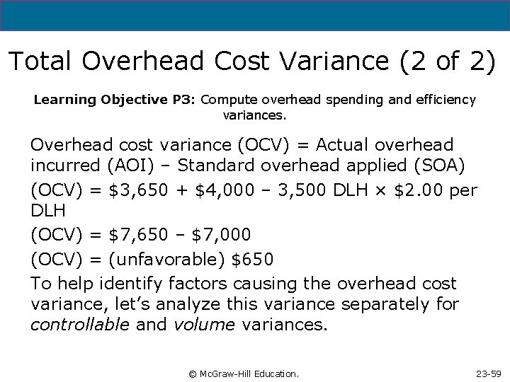
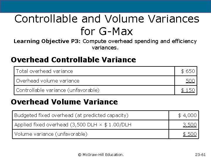
5 - 59 Total Overhead Cost Variance (2 of 2) Learning Objective P 3: Compute overhead spending and efficiency variances. Overhead cost variance (OCV) = Actual overhead incurred (AOI) – Standard overhead applied (SOA) (OCV) = $3, 650 + $4, 000 – 3, 500 DLH × $2. 00 per DLH (OCV) = $7, 650 – $7, 000 (OCV) = (unfavorable) $650 To help identify factors causing the overhead cost variance, let’s analyze this variance separately for controllable and volume variances. © Mc. Graw-Hill Education. 23 -59

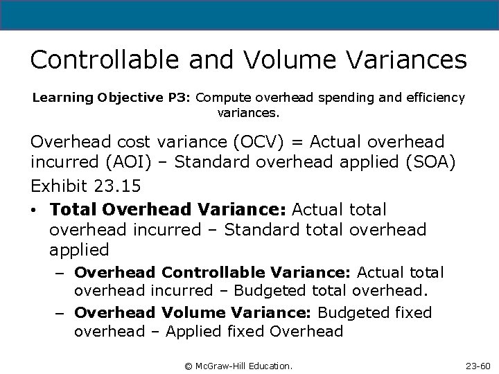
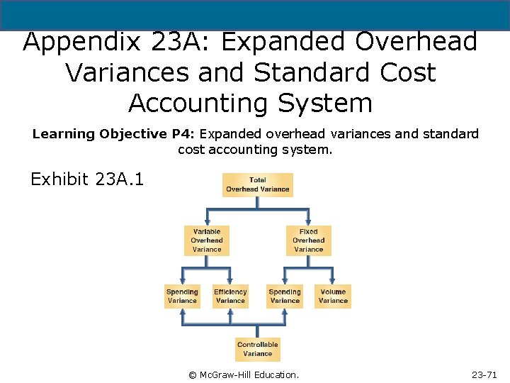
5 - 60 Controllable and Volume Variances Learning Objective P 3: Compute overhead spending and efficiency variances. Overhead cost variance (OCV) = Actual overhead incurred (AOI) – Standard overhead applied (SOA) Exhibit 23. 15 • Total Overhead Variance: Actual total overhead incurred – Standard total overhead applied – Overhead Controllable Variance: Actual total overhead incurred – Budgeted total overhead. – Overhead Volume Variance: Budgeted fixed overhead – Applied fixed Overhead © Mc. Graw-Hill Education. 23 -60

Controllable and Volume Variances for G-Max Learning Objective P 3: Compute overhead spending and efficiency variances. Overhead Controllable Variance Total overhead variance Overhead volume variance Controllable variance (unfavorable) $ 650 500 $ 150 Overhead Volume Variance Budgeted fixed overhead (at predicted capacity) $ 4, 000 Applied fixed overhead (3, 500 DLH × $ 1. 00/DLH 3, 500 Volume variance (unfavorable) $ 500 Copyright © 201 Mc. Graw-Hill Education. All rights reserved. No reproduction or distribution without the prior written consent of Mc. Graw-Hill © Mc. Graw-Hill Education. 23 -61

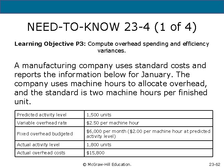
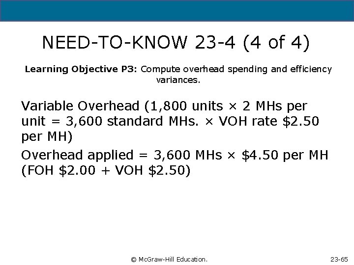
5 - 62 NEED-TO-KNOW 23 -4 (1 of 4) Learning Objective P 3: Compute overhead spending and efficiency variances. A manufacturing company uses standard costs and reports the information below for January. The company uses machine hours to allocate overhead, and the standard is two machine hours per finished unit. Predicted activity level 1, 500 units Variable overhead rate $2. 50 per machine hour Fixed overhead budgeted $6, 000 per month ($2. 00 per machine hour at predicted activity level) Actual activity level 1, 800 units Actual overhead costs $15, 800 © Mc. Graw-Hill Education. 23 -62

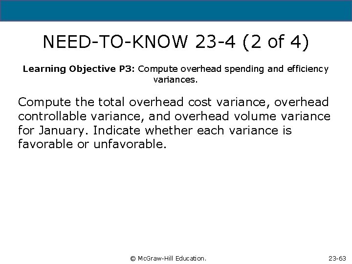
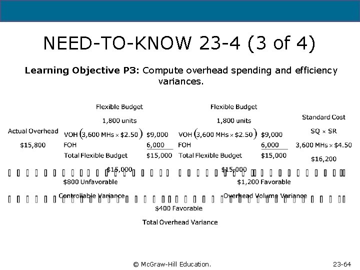
5 - 63 NEED-TO-KNOW 23 -4 (2 of 4) Learning Objective P 3: Compute overhead spending and efficiency variances. Compute the total overhead cost variance, overhead controllable variance, and overhead volume variance for January. Indicate whether each variance is favorable or unfavorable. © Mc. Graw-Hill Education. 23 -63

NEED-TO-KNOW 23 -4 (3 of 4) Learning Objective P 3: Compute overhead spending and efficiency variances. Copyright © 201 Mc. Graw-Hill Education. All rights reserved. No reproduction or distribution without the prior written consent of Mc. Graw-Hill © Mc. Graw-Hill Education. 23 -64

5 - 65 NEED-TO-KNOW 23 -4 (4 of 4) Learning Objective P 3: Compute overhead spending and efficiency variances. Variable Overhead (1, 800 units × 2 MHs per unit = 3, 600 standard MHs. × VOH rate $2. 50 per MH) Overhead applied = 3, 600 MHs × $4. 50 per MH (FOH $2. 00 + VOH $2. 50) © Mc. Graw-Hill Education. 23 -65

5 - 66 Learning Objective A 1: Analyze changes in sales from expected amounts. © Mc. Graw-Hill Education. 23 -66

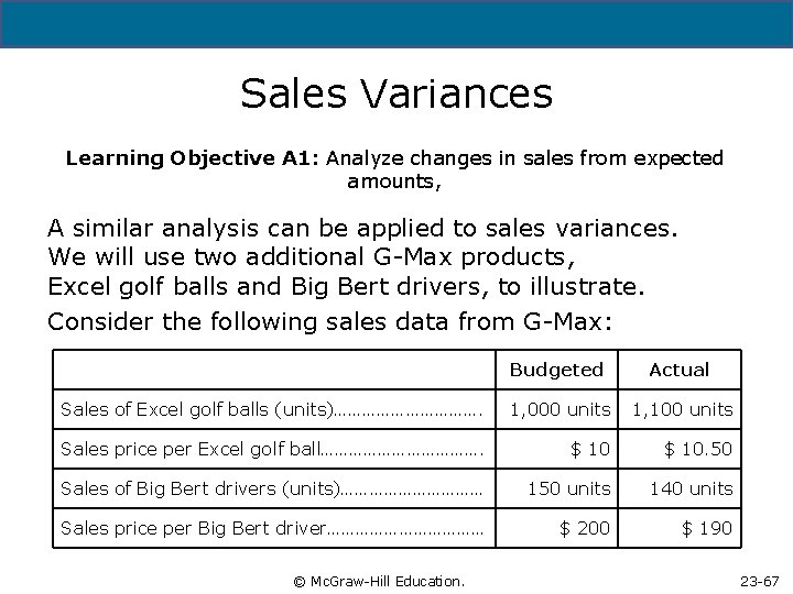
5 - 67 Sales Variances Learning Objective A 1: Analyze changes in sales from expected amounts, A similar analysis can be applied to sales variances. We will use two additional G-Max products, Excel golf balls and Big Bert drivers, to illustrate. Consider the following sales data from G-Max: Budgeted Actual Sales of Excel golf balls (units)……………. 1, 000 units 1, 100 units Sales price per Excel golf ball………………. $ 10. 50 Sales of Big Bert drivers (units)…………… 150 units 140 units Sales price per Big Bert driver……………… $ 200 $ 190 © Mc. Graw-Hill Education. 23 -67

Exhibit 23. 18 Computing Sales Variances for G-Max (1 of 2) Learning Objective A 1: Analyze changes in sales from expected amounts, Copyright © 201 Mc. Graw-Hill Education. All rights reserved. No reproduction or distribution without the prior written consent of Mc. Graw-Hill © Mc. Graw-Hill Education. 23 -68

5 - 69 Exhibit 23. 18 Computing Sales Variances for G-Max (2 of 2) Learning Objective A 1: Analyze changes in sales from expected amounts, *As = actual units; AP= actual sales price; BP = Budgeted sales price: BS = budgeted sales units (fixed budget). © Mc. Graw-Hill Education. 23 -69

5 - 70 Learning Objective P 4 (Appendix): Expanded overhead variances and standard cost accounting system. © Mc. Graw-Hill Education. 23 -70

Appendix 23 A: Expanded Overhead Variances and Standard Cost Accounting System Learning Objective P 4: Expanded overhead variances and standard cost accounting system. Exhibit 23 A. 1 Copyright © 201 Mc. Graw-Hill Education. All rights reserved. No reproduction or distribution without the prior written consent of Mc. Graw-Hill © Mc. Graw-Hill Education. 23 -71

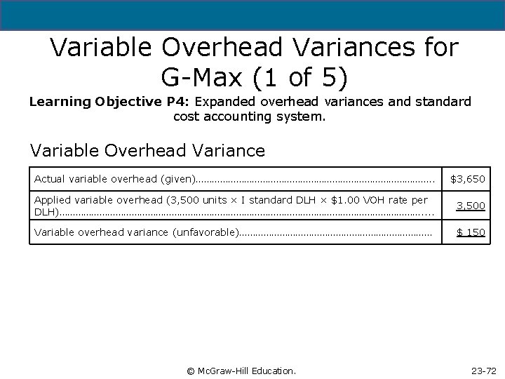
5 - 72 Variable Overhead Variances for G-Max (1 of 5) Learning Objective P 4: Expanded overhead variances and standard cost accounting system. Variable Overhead Variance Actual variable overhead (given)………………………………………. . $3, 650 Applied variable overhead (3, 500 units × I standard DLH × $1. 00 VOH rate per DLH)……………………………………………………………. . 3, 500 Variable overhead variance (unfavorable)……………………………… $ 150 © Mc. Graw-Hill Education. 23 -72

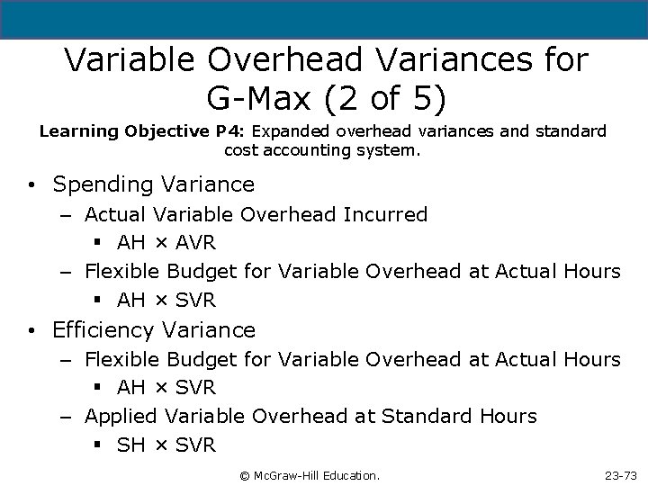
5 - 73 Variable Overhead Variances for G-Max (2 of 5) Learning Objective P 4: Expanded overhead variances and standard cost accounting system. • Spending Variance – Actual Variable Overhead Incurred § AH × AVR – Flexible Budget for Variable Overhead at Actual Hours § AH × SVR • Efficiency Variance – Flexible Budget for Variable Overhead at Actual Hours § AH × SVR – Applied Variable Overhead at Standard Hours § SH × SVR © Mc. Graw-Hill Education. 23 -73

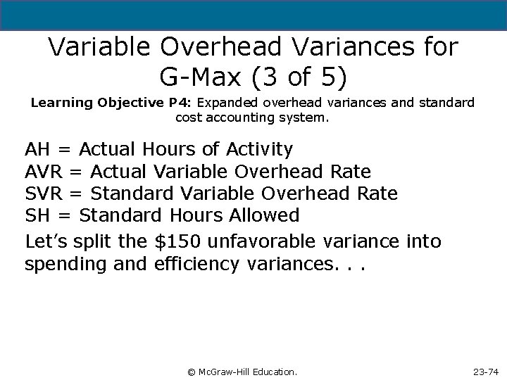
5 - 74 Variable Overhead Variances for G-Max (3 of 5) Learning Objective P 4: Expanded overhead variances and standard cost accounting system. AH = Actual Hours of Activity AVR = Actual Variable Overhead Rate SVR = Standard Variable Overhead Rate SH = Standard Hours Allowed Let’s split the $150 unfavorable variance into spending and efficiency variances. . . © Mc. Graw-Hill Education. 23 -74

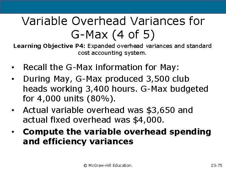
5 - 75 Variable Overhead Variances for G-Max (4 of 5) Learning Objective P 4: Expanded overhead variances and standard cost accounting system. • • Recall the G-Max information for May: During May, G-Max produced 3, 500 club heads working 3, 400 hours. G-Max budgeted for 4, 000 units (80%). Actual variable overhead was $3, 650 and actual fixed overhead was $4, 000. Compute the variable overhead spending and efficiency variances © Mc. Graw-Hill Education. 23 -75

5 - 76 Variable Overhead Variances for G -Max (5 of 5) Learning Objective P 4: Expanded overhead variances and standard cost accounting system. © Mc. Graw-Hill Education. 23 -76

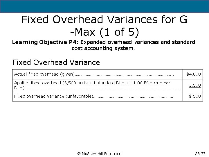
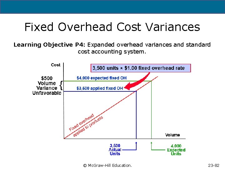
5 - 77 Fixed Overhead Variances for G -Max (1 of 5) Learning Objective P 4: Expanded overhead variances and standard cost accounting system. Fixed Overhead Variance Actual fixed overhead (given)………………………………………. . $4, 000 Applied fixed overhead (3, 500 units × I standard DLH × $1. 00 FOH rate per DLH)……………………………………………………………. . 3, 500 Fixed overhead variance (unfavorable)……………………………… $ 500 © Mc. Graw-Hill Education. 23 -77

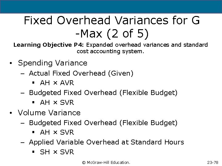
5 - 78 Fixed Overhead Variances for G -Max (2 of 5) Learning Objective P 4: Expanded overhead variances and standard cost accounting system. • Spending Variance – Actual Fixed Overhead (Given) § AH × AVR – Budgeted Fixed Overhead (Flexible Budget) § AH × SVR • Volume Variance – Budgeted Fixed Overhead (Flexible Budget) § AH × SVR – Applied Variable Overhead at Standard Hours § SH × SVR © Mc. Graw-Hill Education. 23 -78

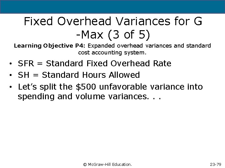
5 - 79 Fixed Overhead Variances for G -Max (3 of 5) Learning Objective P 4: Expanded overhead variances and standard cost accounting system. • SFR = Standard Fixed Overhead Rate • SH = Standard Hours Allowed • Let’s split the $500 unfavorable variance into spending and volume variances. . . © Mc. Graw-Hill Education. 23 -79

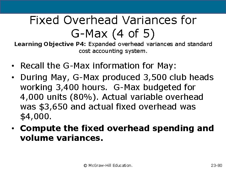
5 - 80 Fixed Overhead Variances for G-Max (4 of 5) Learning Objective P 4: Expanded overhead variances and standard cost accounting system. • Recall the G-Max information for May: • During May, G-Max produced 3, 500 club heads working 3, 400 hours. G-Max budgeted for 4, 000 units (80%). Actual variable overhead was $3, 650 and actual fixed overhead was $4, 000. • Compute the fixed overhead spending and volume variances. © Mc. Graw-Hill Education. 23 -80

Fixed Overhead Variances for G -Max (5 of 5) Learning Objective P 4: Expanded overhead variances and standard cost accounting system. Copyright © 201 Mc. Graw-Hill Education. All rights reserved. No reproduction or distribution without the prior written consent of Mc. Graw-Hill © Mc. Graw-Hill Education. 23 -81

Fixed Overhead Cost Variances Learning Objective P 4: Expanded overhead variances and standard cost accounting system. Copyright © 201 Mc. Graw-Hill Education. All rights reserved. No reproduction or distribution without the prior written consent of Mc. Graw-Hill © Mc. Graw-Hill Education. 23 -82

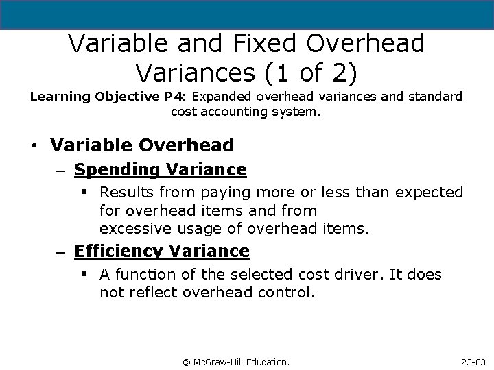
5 - 83 Variable and Fixed Overhead Variances (1 of 2) Learning Objective P 4: Expanded overhead variances and standard cost accounting system. • Variable Overhead – Spending Variance § Results from paying more or less than expected for overhead items and from excessive usage of overhead items. – Efficiency Variance § A function of the selected cost driver. It does not reflect overhead control. © Mc. Graw-Hill Education. 23 -83

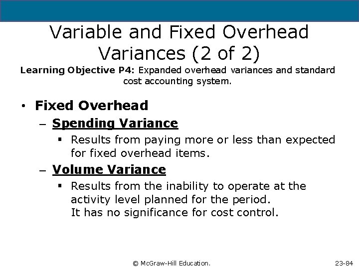
5 - 84 Variable and Fixed Overhead Variances (2 of 2) Learning Objective P 4: Expanded overhead variances and standard cost accounting system. • Fixed Overhead – Spending Variance § Results from paying more or less than expected for fixed overhead items. – Volume Variance § Results from the inability to operate at the activity level planned for the period. It has no significance for cost control. © Mc. Graw-Hill Education. 23 -84

5 - 85 Learning Objective P 5 (Appendix): Prepare journal entries for standard costs and account for price and quantity variances. © Mc. Graw-Hill Education. 23 -85

5 - 86 Standard Cost Accounting System (1 of 5) Learning Objective P 5: Prepare journal entries for standard costs and account for price and quantity variances. • Standard cost systems also record costs and variances in accounts. The entries in the next few slides briefly illustrate the important aspects of this process for G-Max’s standard costs and variances for May. • Recording G-Max material costs for May © Mc. Graw-Hill Education. 23 -86

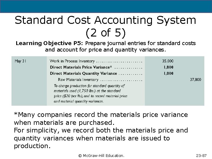
Standard Cost Accounting System (2 of 5) Learning Objective P 5: Prepare journal entries for standard costs and account for price and quantity variances. *Many companies record the materials price variance when materials are purchased. For simplicity, we record both the materials price and quantity variances when materials are issued to production. Copyright © 201 Mc. Graw-Hill Education. All rights reserved. No reproduction or distribution without the prior written consent of Mc. Graw-Hill © Mc. Graw-Hill Education. 23 -87

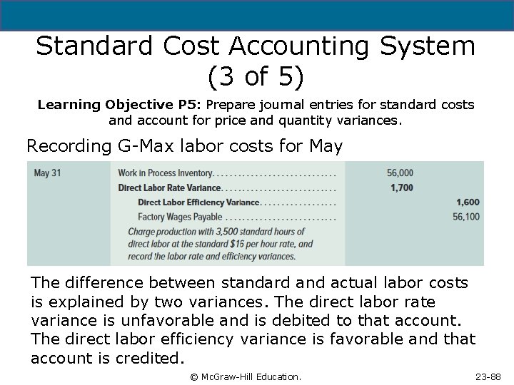
Standard Cost Accounting System (3 of 5) Learning Objective P 5: Prepare journal entries for standard costs and account for price and quantity variances. Recording G-Max labor costs for May The difference between standard and actual labor costs is explained by two variances. The direct labor rate variance is unfavorable and is debited to that account. The direct labor efficiency variance is favorable and that account is credited. Copyright © 201 Mc. Graw-Hill Education. All rights reserved. No reproduction or distribution without the prior written consent of Mc. Graw-Hill © Mc. Graw-Hill Education. 23 -88

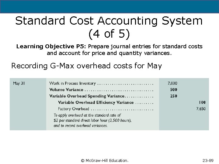
Standard Cost Accounting System (4 of 5) Learning Objective P 5: Prepare journal entries for standard costs and account for price and quantity variances. Recording G-Max overhead costs for May Copyright © 201 Mc. Graw-Hill Education. All rights reserved. No reproduction or distribution without the prior written consent of Mc. Graw-Hill © Mc. Graw-Hill Education. 23 -89

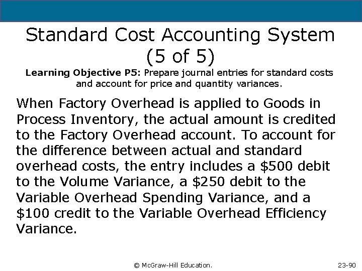
5 - 90 Standard Cost Accounting System (5 of 5) Learning Objective P 5: Prepare journal entries for standard costs and account for price and quantity variances. When Factory Overhead is applied to Goods in Process Inventory, the actual amount is credited to the Factory Overhead account. To account for the difference between actual and standard overhead costs, the entry includes a $500 debit to the Volume Variance, a $250 debit to the Variable Overhead Spending Variance, and a $100 credit to the Variable Overhead Efficiency Variance. © Mc. Graw-Hill Education. 23 -90

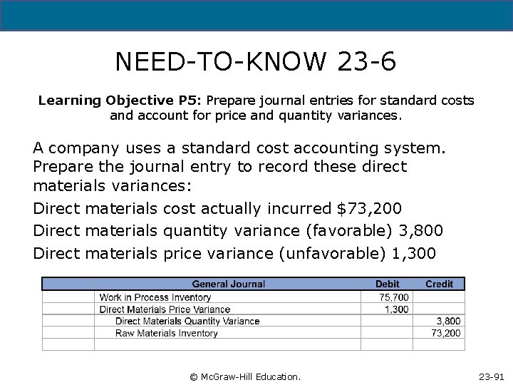
5 - 91 NEED-TO-KNOW 23 -6 Learning Objective P 5: Prepare journal entries for standard costs and account for price and quantity variances. A company uses a standard cost accounting system. Prepare the journal entry to record these direct materials variances: Direct materials cost actually incurred $73, 200 Direct materials quantity variance (favorable) 3, 800 Direct materials price variance (unfavorable) 1, 300 © Mc. Graw-Hill Education. 23 -91

5 - 92 End of Presentation © Mc. Graw-Hill Education. All rights reserved. Authorized only for instructor use in the classroom. No reproduction or further distribution permitted without the prior written consent of Mc. Graw-Hill Education. 23 -92