Functional Verification IV Revisiting Loop Invariants Software Testing

Functional Verification IV: Revisiting Loop Invariants Software Testing and Verification Lecture Notes 24 Prepared by Stephen M. Thebaut, Ph. D. University of Florida

Last Time… • Iteration Recursion Lemma (IRL) • Termination predicate: term(f, P) • Correctness conditions for while_do statement • Sufficient correctness conditions • Correctness conditions for repeat_until statement • Subgoal Induction

Today’s Topics • Thinking about invariants again • Invariant Status Theorem (IST) • While Loop Initialization • Utility of IST

Thinking about invariants again • In Lecture Notes #18 we considered heuristics for synthesizing Q-adequate loop invariants. • In Lecture Notes #23, it was observed that a loop computing a function maintains an important property of state across iterations: the function value of the current state, X, is the same as the function value of the initial state, X 0. That is: f(X)=f(X 0). • We now expand on this observation and show that this property represents the weakest f-adequate loop invariant† over D(f)! † To be defined shortly. . .

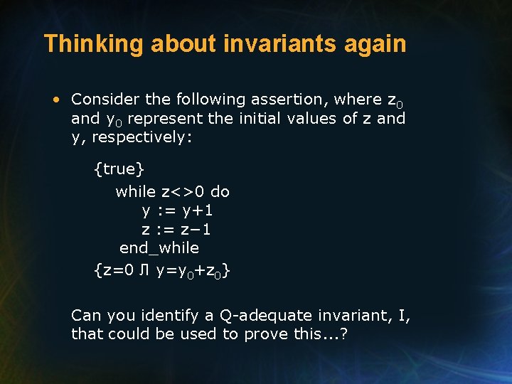
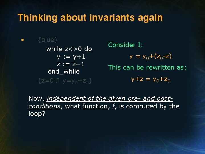
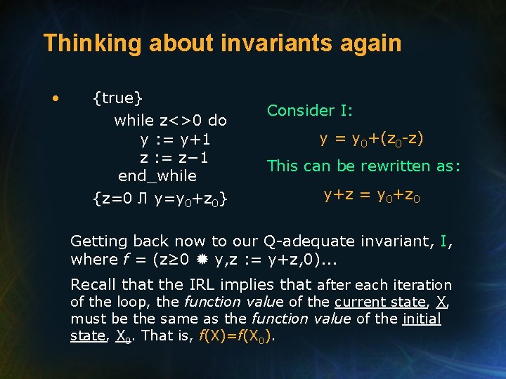
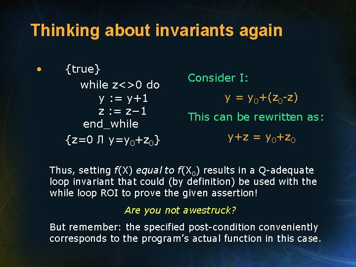
Thinking about invariants again • Consider the following assertion, where z 0 and y 0 represent the initial values of z and y, respectively: {true} while z<>0 do y : = y+1 z : = z− 1 end_while {z=0 Л y=y 0+z 0} Can you identify a Q-adequate invariant, I, that could be used to prove this. . . ?

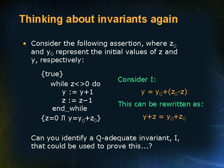
Thinking about invariants again • Consider the following assertion, where z 0 and y 0 represent the initial values of z and y, respectively: {true} while z<>0 do y : = y+1 z : = z− 1 end_while {z=0 Л y=y 0+z 0} Consider I: y = y 0+(z 0 -z) This can be rewritten as: y+z = y 0+z 0 Can you identify a Q-adequate invariant, I, that could be used to prove this. . . ?

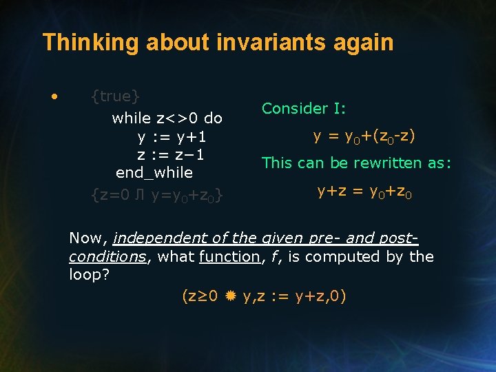
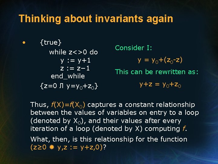
Thinking about invariants again • {true} while z<>0 do y : = y+1 z : = z− 1 end_while {z=0 Л y=y 0+z 0} Consider I: y = y 0+(z 0 -z) This can be rewritten as: y+z = y 0+z 0 Now, independent of the given pre- and postconditions, what function, f, is computed by the loop?

Thinking about invariants again • {true} while z<>0 do y : = y+1 z : = z− 1 end_while {z=0 Л y=y 0+z 0} Consider I: y = y 0+(z 0 -z) This can be rewritten as: y+z = y 0+z 0 Now, independent of the given pre- and postconditions, what function, f, is computed by the loop? (z≥ 0 y, z : = y+z, 0)

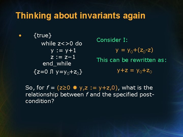
Thinking about invariants again • {true} while z<>0 do y : = y+1 z : = z− 1 end_while {z=0 Л y=y 0+z 0} Consider I: y = y 0+(z 0 -z) This can be rewritten as: y+z = y 0+z 0 So, for f = (z≥ 0 y, z : = y+z, 0), what is the relationship between f and the specified postcondition?

Thinking about invariants again • {true} while z<>0 do y : = y+1 z : = z− 1 end_while {z=0 Л y=y 0+z 0} Consider I: y = y 0+(z 0 -z) This can be rewritten as: y+z = y 0+z 0 So, for f = (z≥ 0 y, z : = y+z, 0), what is the relationship between f and the specified postcondition? z=fz(X 0)=0 Л y=fy(X 0)=y 0+z 0. (This can be written more simply as just X=f(X 0), where “X” is shorthand for “y, z”. )

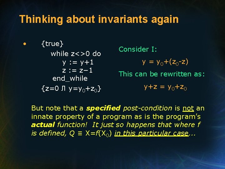
Thinking about invariants again • {true} while z<>0 do y : = y+1 z : = z− 1 end_while {z=0 Л y=y 0+z 0} Consider I: y = y 0+(z 0 -z) This can be rewritten as: y+z = y 0+z 0 But note that a specified post-condition is not an innate property of a program as is the program’s actual function! It just so happens that where f is defined, Q ≡ X=f(X 0) in this particular case. . .

Thinking about invariants again • {true} while z<>0 do y : = y+1 z : = z− 1 end_while {z=0 Л y=y 0+z 0} Consider I: y = y 0+(z 0 -z) This can be rewritten as: y+z = y 0+z 0 Getting back now to our Q-adequate invariant, I, where f = (z≥ 0 y, z : = y+z, 0). . . Recall that the IRL implies that after each iteration of the loop, the function value of the current state, X, must be the same as the function value of the initial state, X 0. That is, f(X)=f(X 0).

Thinking about invariants again • {true} while z<>0 do y : = y+1 z : = z− 1 end_while {z=0 Л y=y 0+z 0} Consider I: y = y 0+(z 0 -z) This can be rewritten as: y+z = y 0+z 0 Thus, f(X)=f(X 0) captures a constant relationship between the values of variables on entry to a loop (denoted by X 0), and their values after every iteration of a loop (denoted by X) computing f. What, then, is this relationship for the function (z≥ 0 y, z : = y+z, 0)?

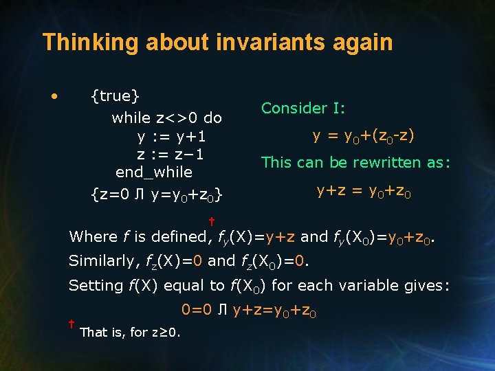
Thinking about invariants again • {true} while z<>0 do y : = y+1 z : = z− 1 end_while {z=0 Л y=y 0+z 0} Consider I: y = y 0+(z 0 -z) This can be rewritten as: y+z = y 0+z 0 † Where f is defined, fy(X)=y+z and fy(X 0)=y 0+z 0. Similarly, fz(X)=0 and fz(X 0)=0. Setting f(X) equal to f(X 0) for each variable gives: † 0=0 Л y+z=y 0+z 0 That is, for z≥ 0.

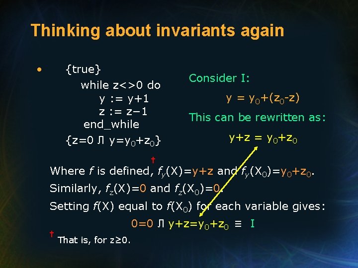
Thinking about invariants again • {true} while z<>0 do y : = y+1 z : = z− 1 end_while {z=0 Л y=y 0+z 0} Consider I: y = y 0+(z 0 -z) This can be rewritten as: y+z = y 0+z 0 † Where f is defined, fy(X)=y+z and fy(X 0)=y 0+z 0. Similarly, fz(X)=0 and fz(X 0)=0. Setting f(X) equal to f(X 0) for each variable gives: † 0=0 Л y+z=y 0+z 0 ≡ I That is, for z≥ 0.

Thinking about invariants again • {true} while z<>0 do y : = y+1 z : = z− 1 end_while {z=0 Л y=y 0+z 0} Consider I: y = y 0+(z 0 -z) This can be rewritten as: y+z = y 0+z 0 Thus, setting f(X) equal to f(X 0) results in a Q-adequate loop invariant that could (by definition) be used with the while loop ROI to prove the given assertion! Are you not awestruck? But remember: the specified post-condition conveniently corresponds to the program’s actual function in this case.

Invariant Status Theorem (IST) • Theorem. Let f = [while p do g]. If X 0 D(f), X D(f), and q(X)=( f(X)=f(X 0) ), then q is an invariant of while p do g; i. e. , it has the following properties: 1. 2. q(X 0) is true, and ( q(X) Л p(X) ) qog(X). In addition, q(X) is an f-adequate invariant; i. e. , 3. ( q(X) Л ¬p(X) ) ( X=f(X 0) ) This represents the final state values as a function, f, of the initial state values.

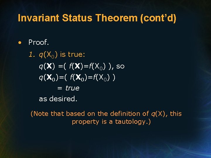
Invariant Status Theorem (cont’d) • Proof. 1. q(X 0) is true: q(X) =( f(X)=f(X 0) ), so q(X 0)=( f(X 0)=f(X 0) ) = true as desired. (Note that based on the definition of q(X), this property is a tautology. )

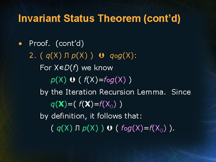
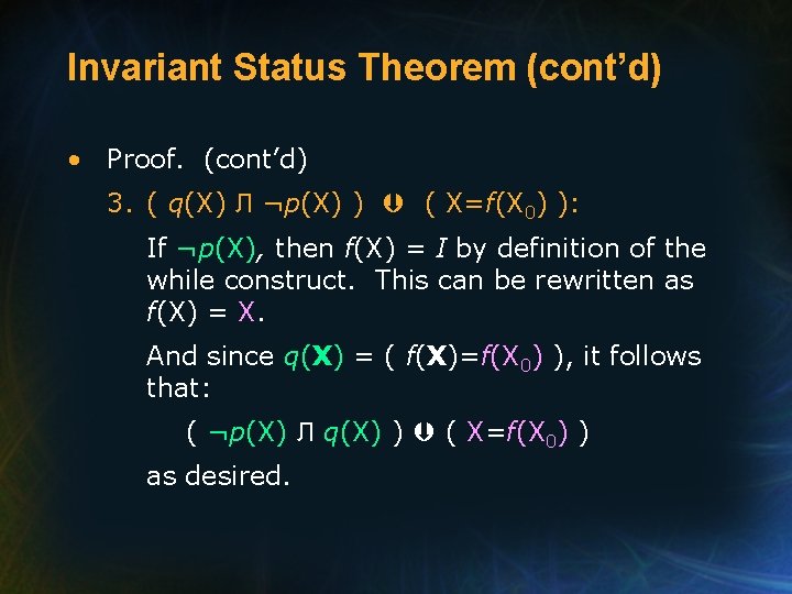
Invariant Status Theorem (cont’d) • Proof. (cont’d) 2. ( q(X) Л p(X) ) qog(X): For X D(f) we know p(X) ( f(X)=fog(X) ) by the Iteration Recursion Lemma. Since q(X)=( f(X)=f(X 0) ) by definition, it follows that: ( q(X) Л p(X) ) ( fog(X)=f(X 0) ).

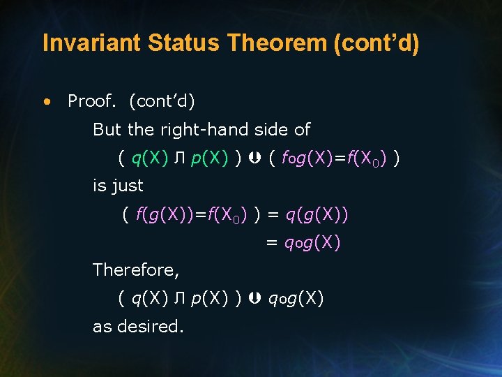
Invariant Status Theorem (cont’d) • Proof. (cont’d) But the right-hand side of ( q(X) Л p(X) ) ( fog(X)=f(X 0) ) is just ( f(g(X))=f(X 0) ) = q(g(X)) = qog(X) Therefore, ( q(X) Л p(X) ) qog(X) as desired.

Invariant Status Theorem (cont’d) • Proof. (cont’d) 3. ( q(X) Л ¬p(X) ) ( X=f(X 0) ): If ¬p(X), then f(X) = I by definition of the while construct. This can be rewritten as f(X) = X. And since q(X) = ( f(X)=f(X 0) ), it follows that: ( ¬p(X) Л q(X) ) ( X=f(X 0) ) as desired.

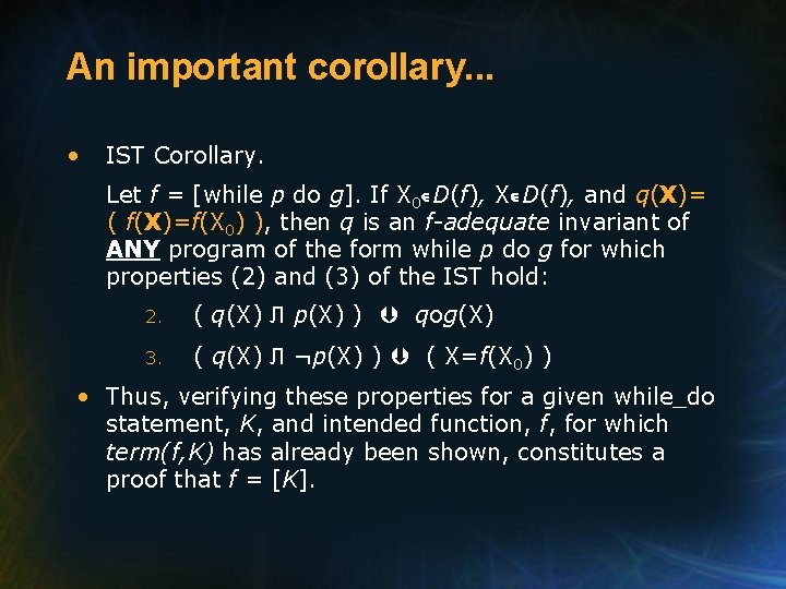
An important corollary. . . • IST Corollary. Let f = [while p do g]. If X 0 D(f), X D(f), and q(X)= ( f(X)=f(X 0) ), then q is an f-adequate invariant of ANY program of the form while p do g for which properties (2) and (3) of the IST hold: 2. ( q(X) Л p(X) ) qog(X) 3. ( q(X) Л ¬p(X) ) ( X=f(X 0) ) • Thus, verifying these properties for a given while_do statement, K, and intended function, f, for which term(f, K) has already been shown, constitutes a proof that f = [K].

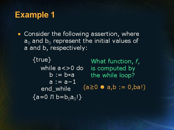
Example 1 • Consider the following assertion, where a 0 and b 0 represent the initial values of a and b, respectively: {true} What function, f, while a<>0 do is computed by b : = b*a the while loop? a : = a− 1 (a≥ 0 a, b : = 0, ba!) end_while {a=0 Л b=b 0 a 0!}

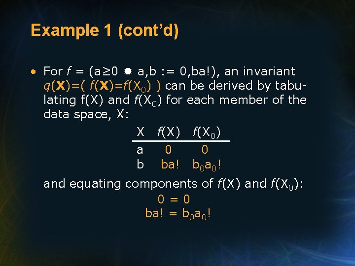
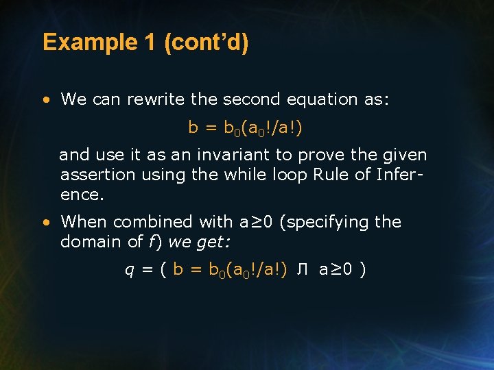
Example 1 (cont’d) • For f = (a≥ 0 a, b : = 0, ba!), an invariant q(X)=( f(X)=f(X 0) ) can be derived by tabulating f(X) and f(X 0) for each member of the data space, X: X f(X) f(X 0) a 0 0 b ba! b 0 a 0! and equating components of f(X) and f(X 0): 0=0 ba! = b 0 a 0!

Example 1 (cont’d) • We can rewrite the second equation as: b = b 0(a 0!/a!) and use it as an invariant to prove the given assertion using the while loop Rule of Inference. • When combined with a≥ 0 (specifying the domain of f) we get: q = ( b = b 0(a 0!/a!) Л a≥ 0 )

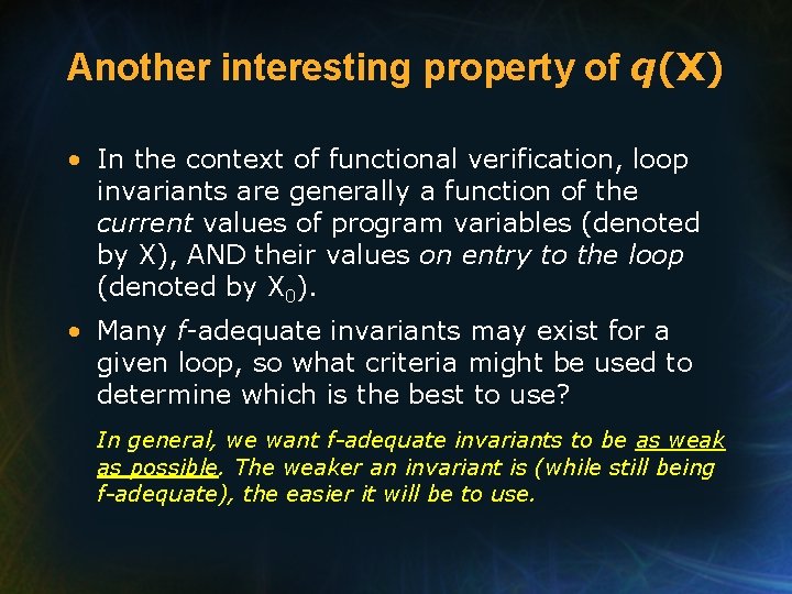
Another interesting property of q(X) • In the context of functional verification, loop invariants are generally a function of the current values of program variables (denoted by X), AND their values on entry to the loop (denoted by X 0). • Many f-adequate invariants may exist for a given loop, so what criteria might be used to determine which is the best to use? In general, we want f-adequate invariants to be as weak as possible. The weaker an invariant is (while still being f-adequate), the easier it will be to use.

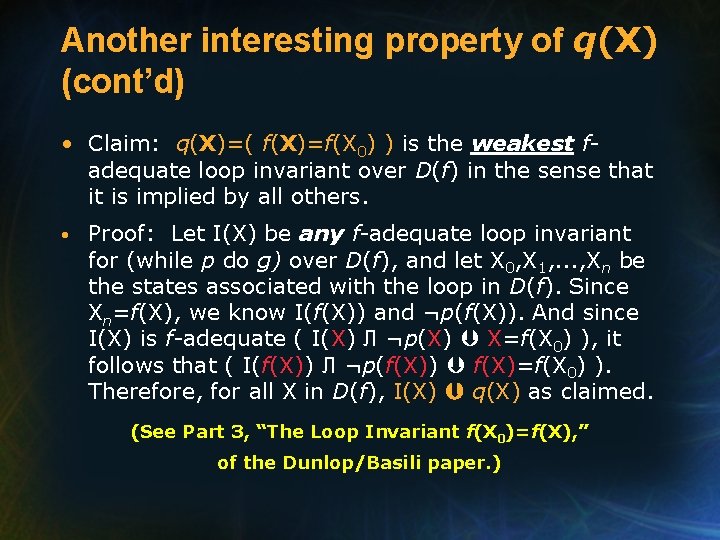
Another interesting property of q(X) (cont’d) • Claim: q(X)=( f(X)=f(X 0) ) is the weakest fadequate loop invariant over D(f) in the sense that it is implied by all others. • Proof: Let I(X) be any f-adequate loop invariant for (while p do g) over D(f), and let X 0, X 1, . . . , Xn be the states associated with the loop in D(f). Since Xn=f(X), we know I(f(X)) and ¬p(f(X)). And since I(X) is f-adequate ( I(X) Л ¬p(X) X=f(X 0) ), it follows that ( I(f(X)) Л ¬p(f(X)) f(X)=f(X 0) ). Therefore, for all X in D(f), I(X) q(X) as claimed. (See Part 3, “The Loop Invariant f(X 0)=f(X), ” of the Dunlop/Basili paper. )

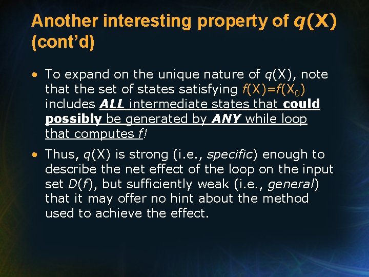
Another interesting property of q(X) (cont’d) • To expand on the unique nature of q(X), note that the set of states satisfying f(X)=f(X 0) includes ALL intermediate states that could possibly be generated by ANY while loop that computes f! • Thus, q(X) is strong (i. e. , specific) enough to describe the net effect of the loop on the input set D(f), but sufficiently weak (i. e. , general) that it may offer no hint about the method used to achieve the effect.

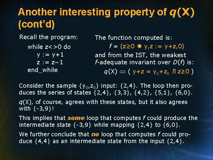
Another interesting property of q(X) (cont’d) Recall the program: while z<>0 do y : = y+1 z : = z− 1 end_while The function computed is: f = (z≥ 0 y, z : = y+z, 0) and from the IST, the weakest f-adequate invariant over D(f) is: q(X) ( y+z = y 0+z 0 Л z≥ 0 ) Consider the sample {y 0, z 0} input: {2, 4}. The loop then produces the series of states {2, 4}, {3, 3}, {4, 2}, {5, 1}, {6, 0}. q(X), of course, agrees with these states, but it also agrees with {-3, 9}! This implies that some loop that computes f could produce the intermediate state {-3, 9} while mapping {2, 4} to {6, 0}. We further conclude that no loop that computes f could produce {4, 4} as an intermediate state from the input {2, 4}.

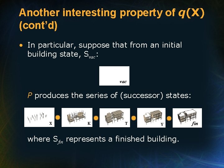
Another interesting property of q(X) (cont’d) • Consider a more “concrete” (wood, aluminum, etc. ) illustration of q’s properties. . . • Let f represent a general mapping from an initial building construction state (e. g. , a vacant lot) to a final construction state (a finished building). • Let P be a specific, step-by-step, iterative construction process that produces a finished building in accordance with f.

Another interesting property of q(X) (cont’d) • In particular, suppose that from an initial building state, Svac: vac P produces the series of (successor) states: X K T Y where Sfin represents a finished building. fin

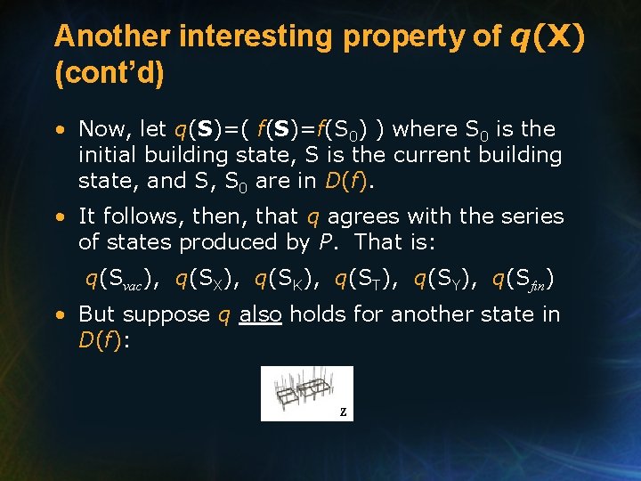
Another interesting property of q(X) (cont’d) • Now, let q(S)=( f(S)=f(S 0) ) where S 0 is the initial building state, S is the current building state, and S, S 0 are in D(f). • It follows, then, that q agrees with the series of states produced by P. That is: q(Svac), q(SX), q(SK), q(ST), q(SY), q(Sfin) • But suppose q also holds for another state in D(f): Z

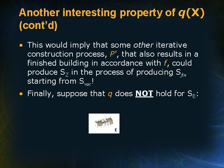
Another interesting property of q(X) (cont’d) • This would imply that some other iterative construction process, P’, that also results in a finished building in accordance with f, could produce SZ in the process of producing Sfin starting from Svac! • Finally, suppose that q does NOT hold for SE: E

Another interesting property of q(X) (cont’d) • This would imply that no iterative construction process that results in a finished building in accordance with f could produce SE from the initial state Svac!

Today’s Topics • Thinking about invariants again • Invariant Status Theorem (IST) • While Loop Initialization • Utility of IST

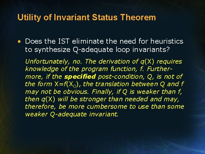
Utility of Invariant Status Theorem • Does the IST eliminate the need for heuristics to synthesize Q-adequate loop invariants? Unfortunately, no. The derivation of q(X) requires knowledge of the program function, f. Furthermore, if the specified post-condition, Q, is not of the form X=f(X 0), the translation between Q and f may not be obvious. Finally, if Q is weaker than f, then q(X) will be stronger than needed and may, therefore, be more cumbersome to use than some weaker Q-adequate invariant.

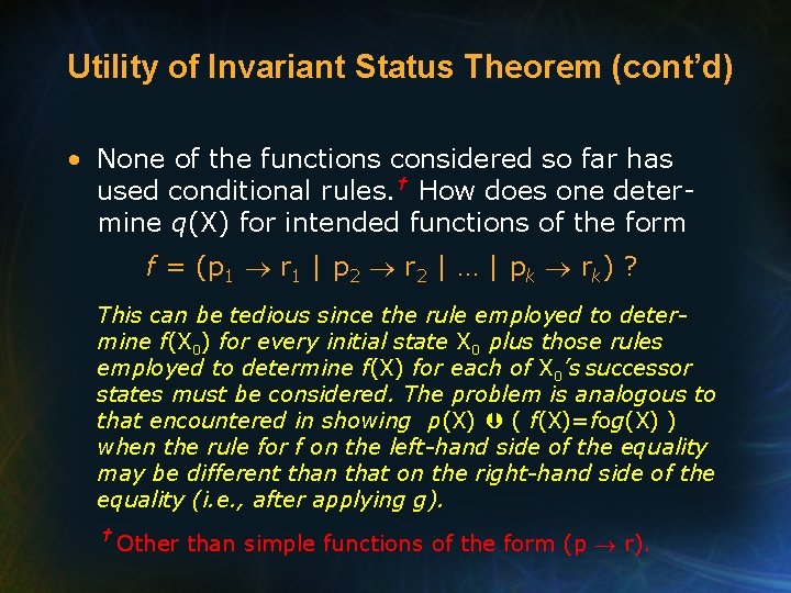
Utility of Invariant Status Theorem (cont’d) • None of the functions considered so far has used conditional rules. † How does one determine q(X) for intended functions of the form f = (p 1 r 1 | p 2 r 2 | … | pk rk) ? This can be tedious since the rule employed to determine f(X 0) for every initial state X 0 plus those rules employed to determine f(X) for each of X 0’s successor states must be considered. The problem is analogous to that encountered in showing p(X) ( f(X)=fog(X) ) when the rule for f on the left-hand side of the equality may be different than that on the right-hand side of the equality (i. e. , after applying g). † Other than simple functions of the form (p r).

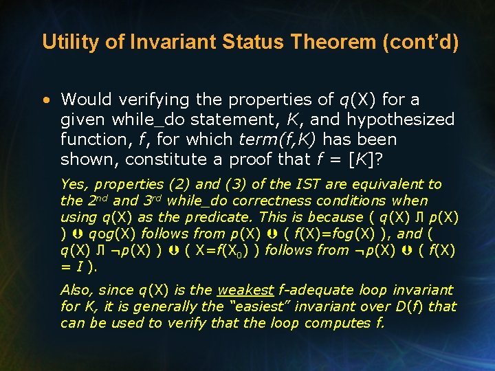
Utility of Invariant Status Theorem (cont’d) • Would verifying the properties of q(X) for a given while_do statement, K, and hypothesized function, f, for which term(f, K) has been shown, constitute a proof that f = [K]? Yes, properties (2) and (3) of the IST are equivalent to the 2 nd and 3 rd while_do correctness conditions when using q(X) as the predicate. This is because ( q(X) Л p(X) ) qog(X) follows from p(X) ( f(X)=fog(X) ), and ( q(X) Л ¬p(X) ) ( X=f(X 0) ) follows from ¬p(X) ( f(X) = I ). Also, since q(X) is the weakest f-adequate loop invariant for K, it is generally the “easiest” invariant over D(f) that can be used to verify that the loop computes f.

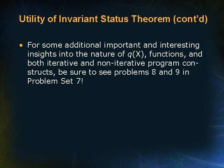
Utility of Invariant Status Theorem (cont’d) • For some additional important and interesting insights into the nature of q(X), functions, and both iterative and non-iterative program constructs, be sure to see problems 8 and 9 in Problem Set 7!

Summary • Thinking about invariants again • Invariant Status Theorem (IST) • While Loop Initialization • Utility of IST

Functional Verification IV: Revisiting Loop Invariants Software Testing and Verification Lecture Notes 24 Prepared by Stephen M. Thebaut, Ph. D. University of Florida