FUNCTIONAL FORMS OF REGRESSION MODELS A functional form

FUNCTIONAL FORMS OF REGRESSION MODELS • A functional form refers to the algebraic form of the relationship between a dependent variable and the regressor(s). • The simplest functional form is the linear functional form, where the relationship between the dependent variable and an independent variable is graphically represented by a straight line. 7 -0

EXAMPLES • Linear models • The log-linear model • Semilog models • Reciprocal models • The logarithmic reciprocal model © 2011 Pearson Addison-Wesley. All rights reserved. 7 -1

Choosing a Functional Form • After the independent variables are chosen, the next step is to choose the functional form of the relationship between the dependent variable and each of the independent variables. • Let theory be your guide! Not the data! © 2011 Pearson Addison-Wesley. All rights reserved. 7 -2

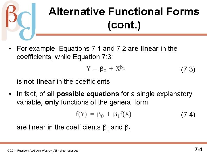
Alternative Functional Forms • An equation is linear in the variables if plotting the function in terms of X and Y generates a straight line • For example, Equation 7. 1: Y = β 0 + β 1 X + ε (7. 1) is linear in the variables but Equation 7. 2: Y = β 0 + β 1 X 2 + ε (7. 2) is not linear in the variables • Similarly, an equation is linear in the coefficients only if the coefficients appear in their simplest form—they: – are not raised to any powers (other than one) – are not multiplied or divided by other coefficients – do not themselves include some sort of function (like logs or exponents) © 2011 Pearson Addison-Wesley. All rights reserved. 7 -3

Alternative Functional Forms (cont. ) • For example, Equations 7. 1 and 7. 2 are linear in the coefficients, while Equation 7: 3: (7. 3) is not linear in the coefficients • In fact, of all possible equations for a single explanatory variable, only functions of the general form: (7. 4) are linear in the coefficients β 0 and β 1 © 2011 Pearson Addison-Wesley. All rights reserved. 7 -4

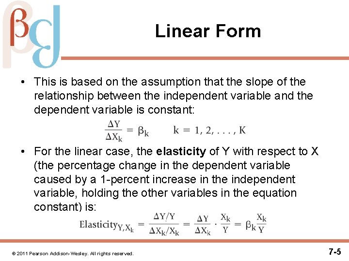
Linear Form • This is based on the assumption that the slope of the relationship between the independent variable and the dependent variable is constant: • For the linear case, the elasticity of Y with respect to X (the percentage change in the dependent variable caused by a 1 -percent increase in the independent variable, holding the other variables in the equation constant) is: © 2011 Pearson Addison-Wesley. All rights reserved. 7 -5

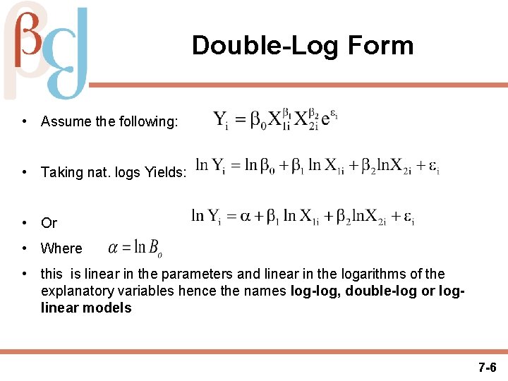
Double-Log Form • Assume the following: • Taking nat. logs Yields: • Or • Where • this is linear in the parameters and linear in the logarithms of the explanatory variables hence the names log-log, double-log or loglinear models 7 -6

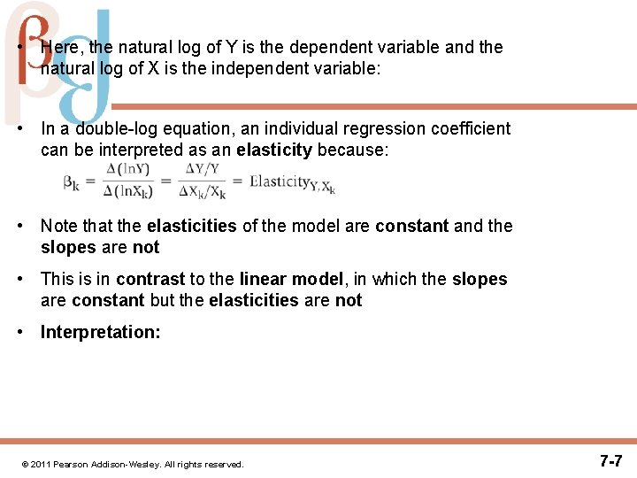
• Here, the natural log of Y is the dependent variable and the natural log of X is the independent variable: • In a double-log equation, an individual regression coefficient can be interpreted as an elasticity because: • Note that the elasticities of the model are constant and the slopes are not • This is in contrast to the linear model, in which the slopes are constant but the elasticities are not • Interpretation: © 2011 Pearson Addison-Wesley. All rights reserved. 7 -7

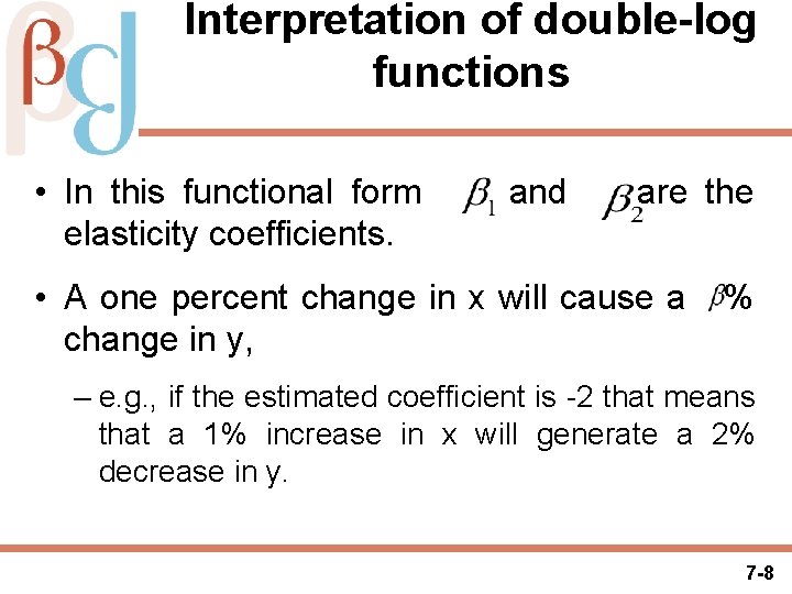
Interpretation of double-log functions • In this functional form and are the elasticity coefficients. • A one percent change in x will cause a % change in y, – e. g. , if the estimated coefficient is -2 that means that a 1% increase in x will generate a 2% decrease in y. 7 -8

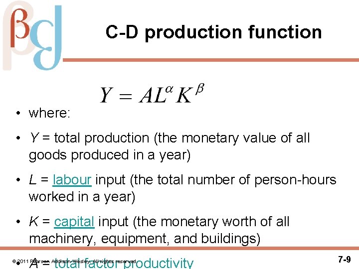
C-D production function • where: • Y = total production (the monetary value of all goods produced in a year) • L = labour input (the total number of person-hours worked in a year) • K = capital input (the monetary worth of all machinery, equipment, and buildings) • A = total factor productivity © 2011 Pearson Addison-Wesley. All rights reserved. 7 -9

• α and β are the output elasticities of labour and capital, respectively. These values are constants determined by available technology. • Output elasticity measures the responsiveness of output to a change in levels of either labour or capital used in production, ceteris paribus. For example if α = 0. 15, a 1% increase in labour would lead to approximately a 0. 15% increase in output. • Further, if: • α + β = 1, the production function has constant returns to scale: Doubling capital K and labour L will also double output Y. If • α + β < 1, returns to scale are decreasing, and if • α + β > 1 returns to scale are increasing. © 2011 Pearson Addison-Wesley. All rights reserved. 7 -10

Semilog Form • The semilog functional form is a variant of the doublelog equation in which some but not all of the variables (dependent and independent) are expressed in terms of their natural logs. • It can be on the right-hand side, as in: lin-log model: Yi = β 0 + β 1 ln. X 1 i + β 2 X 2 i + εi (7. 7) • Or it can be on the left-hand side, as in: log-lin: ln. Y = β 0 + β 1 X 1 + β 2 X 2 + ε (7. 9) 7 -11

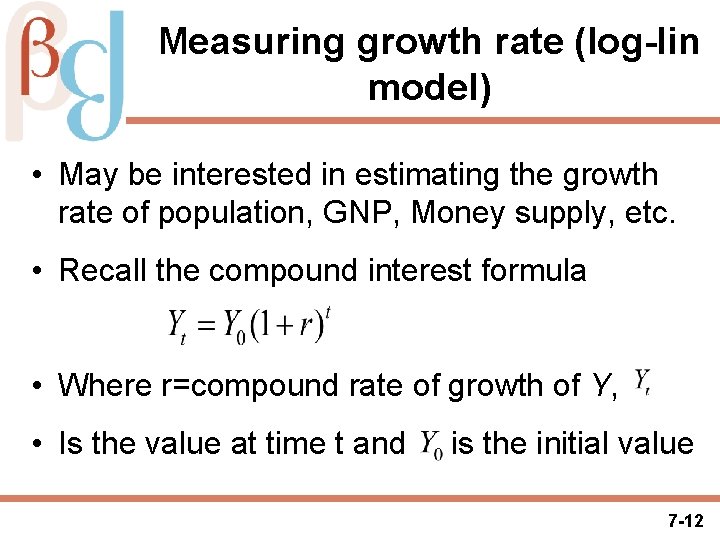
Measuring growth rate (log-lin model) • May be interested in estimating the growth rate of population, GNP, Money supply, etc. • Recall the compound interest formula • Where r=compound rate of growth of Y, • Is the value at time t and is the initial value 7 -12

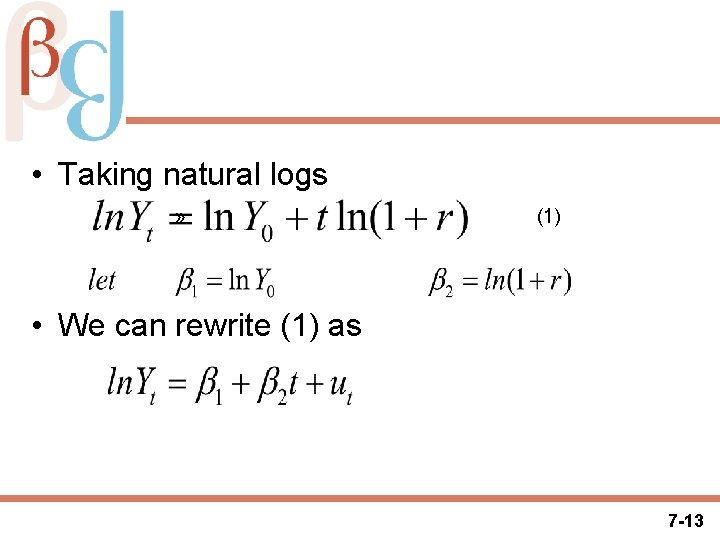
• Taking natural logs » (1) • We can rewrite (1) as 7 -13

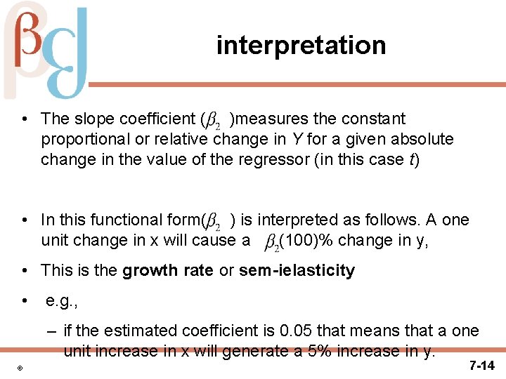
interpretation • The slope coefficient ( )measures the constant proportional or relative change in Y for a given absolute change in the value of the regressor (in this case t) • In this functional form( ) is interpreted as follows. A one unit change in x will cause a (100)% change in y, • This is the growth rate or sem-ielasticity • e. g. , – if the estimated coefficient is 0. 05 that means that a one unit increase in x will generate a 5% increase in y. © 7 -14

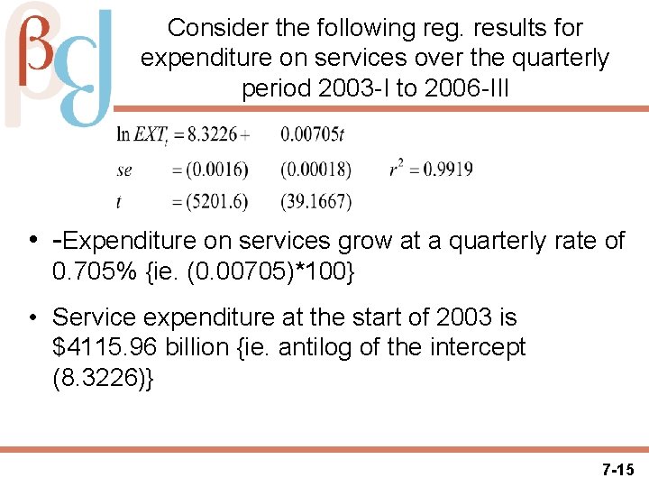
Consider the following reg. results for expenditure on services over the quarterly period 2003 -I to 2006 -III • -Expenditure on services grow at a quarterly rate of 0. 705% {ie. (0. 00705)*100} • Service expenditure at the start of 2003 is $4115. 96 billion {ie. antilog of the intercept (8. 3226)} 7 -15

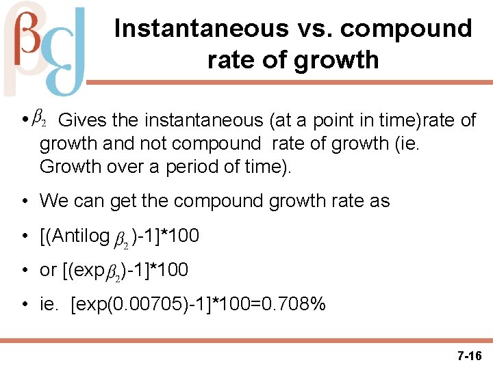
Instantaneous vs. compound rate of growth • Gives the instantaneous (at a point in time)rate of growth and not compound rate of growth (ie. Growth over a period of time). • We can get the compound growth rate as • [(Antilog )-1]*100 • or [(exp )-1]*100 • ie. [exp(0. 00705)-1]*100=0. 708% 7 -16

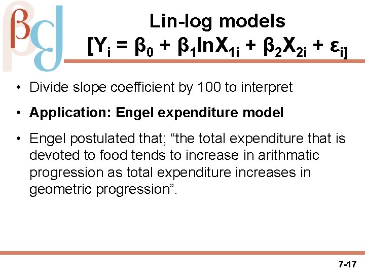
Lin-log models [Yi = β 0 + β 1 ln. X 1 i + β 2 X 2 i + εi] • Divide slope coefficient by 100 to interpret • Application: Engel expenditure model • Engel postulated that; “the total expenditure that is devoted to food tends to increase in arithmatic progression as total expenditure increases in geometric progression”. 7 -17

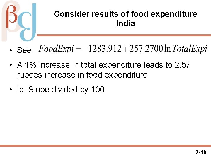
Consider results of food expenditure India • See • A 1% increase in total expenditure leads to 2. 57 rupees increase in food expenditure • Ie. Slope divided by 100 7 -18

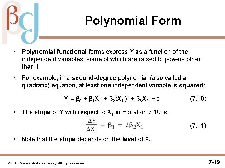
Polynomial Form • Polynomial functional forms express Y as a function of the independent variables, some of which are raised to powers other than 1 • For example, in a second-degree polynomial (also called a quadratic) equation, at least one independent variable is squared: Yi = β 0 + β 1 X 1 i + β 2(X 1 i)2 + β 3 X 2 i + εi (7. 10) • The slope of Y with respect to X 1 in Equation 7. 10 is: (7. 11) • Note that the slope depends on the level of X 1 © 2011 Pearson Addison-Wesley. All rights reserved. 7 -19

Figure 7. 4 Polynomial Functions © 2011 Pearson Addison-Wesley. All rights reserved. 7 -20

Inverse (reciprocal) Form • The inverse functional form expresses Y as a function of the reciprocal (or inverse) of one or more of the independent variables (in this case, X 1): Yi = β 0 + β 1(1/X 1 i) + β 2 X 2 i + εi (7. 13) • So X 1 cannot equal zero • This functional form is relevant when the impact of a particular independent variable is expected to approach zero as that independent variable approaches infinity • The slope with respect to X 1 is: (7. 14) • The slopes for X 1 fall into two categories, depending on the sign of β 1 © 2011 Pearson Addison-Wesley. All rights reserved. 7 -21

Properties of reciprocal forms • As the regressor increases indefinitely the regressand approaches its limiting or asymptotic value (the intercept). 7 -22

Example: relationship b/n child mortality (CM) & per capita GNP (PGNP) • Now • As PGNP increases indefinitely CM reaches its asymptotic value of 82 deaths per thousand. 7 -23

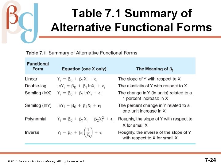
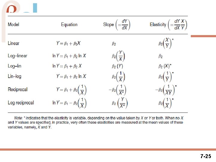
Table 7. 1 Summary of Alternative Functional Forms © 2011 Pearson Addison-Wesley. All rights reserved. 7 -24

7 -25