Functional Dependency and Decomposition INTRODUCTION FUNCTIONAL DEPENDENCY FD

Functional Dependency and Decomposition ØINTRODUCTION ØFUNCTIONAL DEPENDENCY (FD) ØFunctional Dependency Diagram and Examples ØFull Functional Dependency (FFD) ØArmstrong's Axioms for Functional Dependencies ØRedundant Functional Dependencies ØClosures of a Set of Functional Dependencies ØDECOMPOSITION ØLossy Decomposition ØLossless-Join Decomposition ØDependency-Preserving Decomposition

INTRODUCTION • The purpose of database design is to arrange the corporate data fields into an organized structure such that it generates set of relationships and stores information without unnecessary redundancy. • In fact, the redundancy and database consistency are the most important logical criteria in database design. .

FUNCTIONAL DEPENDENCY (FD) • A functional dependency (FD) is a property of the information represented by the relation. • Functional dependency allows the database designer to express facts about the enterprise that the designer is modeling with the enterprise databases. • It allows the designer to express constraints, which cannot be expressed with super keys.

• Functional dependency is a term derived from mathematical theory, which states that for every element in the attribute (which appears on some row), there is a unique corresponding element (on the same row). l. Let us assume that rows (tuples) of a relational table T is represented by the notation r 1 , r 2 , ……. . , and individual attributes (columns) of the table is represented by letters A, B, …. The letters X, Y , …. . , represent the subsets of attributes.

l l Thus, as per mathematical theory, for a given table T containing at least two attributes A and B, we can say that A B. The arrow notation ' ' is read as "functionally determines". Thus, we can say that, A functionally determines B or B is functionally dependent on A. In other words, we can say that, given two rows R 1, and R 2 , in table T, if R 1(A) = R 2(A) then R 1(B) = R 2(B).

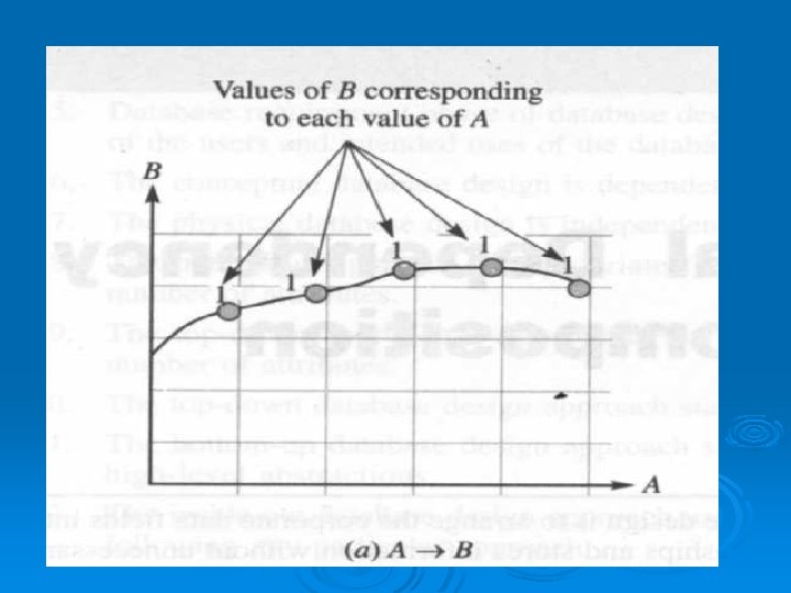
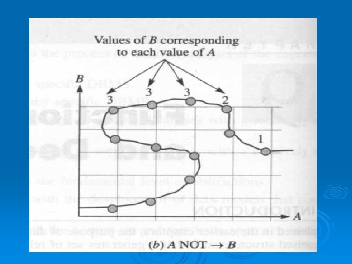
l l l fig illustrates a graphical representation of the functional dependency concept. As shown in Fig. (a) , A functionally determines B. Each value of A corresponds to only one value of B. However, in (b), A does not functionally determine B. Some values of A correspond to more than one value of B The attributes in subset A are sometimes known as the determinant of FD: A B.

l l The left hand side of the functional dependency is sometimes called determinant whereas that of the right hand side is called the dependent. The determinant and dependent are both sets of attributes. A functional dependency is a many-to-one relationship between two sets of attributes X and Y of a given table T. Here X and Y are subsets of the set of attributes of table T. Thus, the functional dependency X Y is said to hold in relation R if and only if, whenever two tuples (rows or records) of T have the same value of X, they also have the same value for Y.

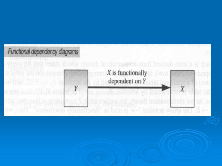
Functional Dependency Diagram and Examples In a functional dependency diagram (FDD), functional dependency is represented by rectangles representing attributes and a heavy arrow showing dependency. Fig. shows a functional dependency diagram for the simplest functional dependency, that is, Ø FD: Y X. Ø

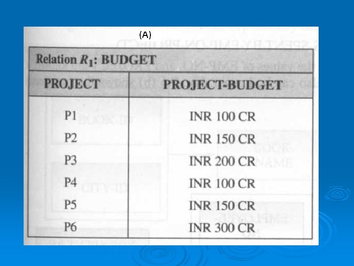
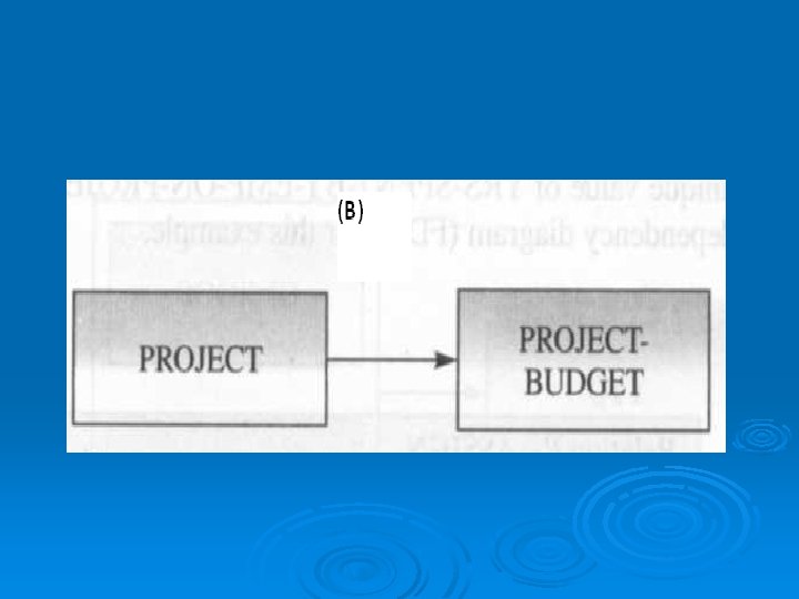
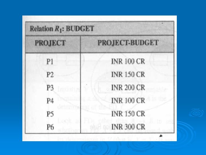
Example 1 • Let us consider a functional dependency of relation R 1: BUDGET, as shown in Fig. (a), which is given as: FD: {PROJECT} {PROJECT-BUDGET}

• It means that in the BUDGET relation (or table), PROJECT-BUDGET is functionally dependent on PROJECT, because each project has one given budget value. • Thus, once a project name is known, a unique value of PROJECT-BUDGET is also immediately known. • Fig. (b) shows the functional dependency diagram (FDD) for this example.

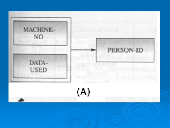
l Example 2 Let us consider a functional dependency that there is one person working on a machine each day, which is given as: FD: {MACHINE-NO, DATE-USED} {PERSON-ID} It means that once the values of MACHINENO and DATE-USED are known, a unique value of PERSON-ID also can be known. Fig. (a) shows the functional dependency diagram (FDD) for this example.

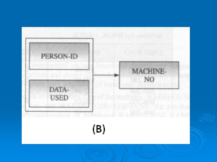
Similarly, in the above example, if the person also uses one machine each day, then FD can be given as: FD: {PERSON-ID, DATE-USED} {MACHINE-NO} It means that once the values of PERSON-ID and DATE-USED are known, a unique value of MACHINE-NO also can be known. Fig. (b) shows the functional dependency diagram (FDD) for this example

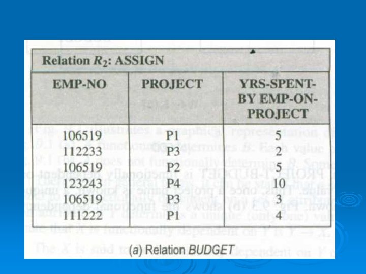
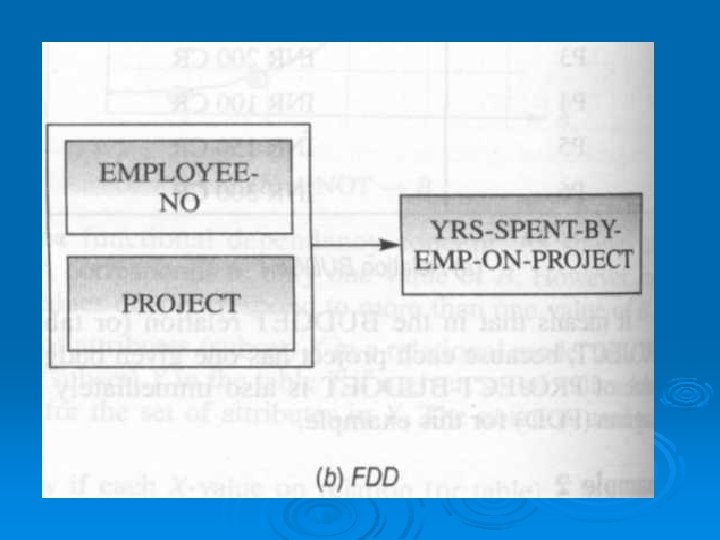
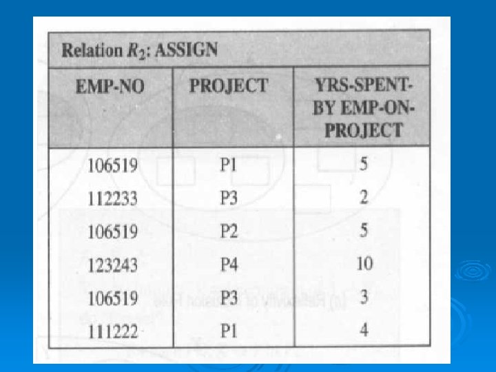
Example 3 Let us consider a functional dependency of relation R 2: ASSIGN, as shown in Fig. (a), which is given as: FD: {EMP-ID, PROJECT) {YRS-SPENT-BY -EMP-ON-PROJECT) It means that in an ASSIGN relation (or table), once the values of EMP-NO. and PROJECT are known, a unique value of YRS-SPENT-B Y-EMP-ON-PROJECT also can be known. Fig. (b) shows the functional dependency diagram (FDD) for this example.

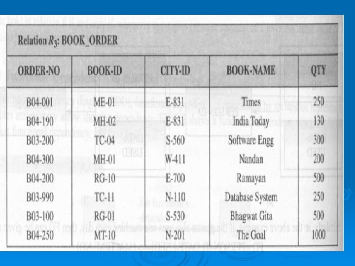
Example 4 • Let us consider a functional dependency of relation R 3: BOOK_ORDER, as shown in Fig. satisfies several functional dependencies, which can be given as: • FD: {BOOK-ID, CITY-ID} {BOOK-NAME} • FD: {BOOK-ID, CITY-ID} {QTY} • FD: {BOOK-ID, CITY-ID} NAME} {QTY, BOOK-

In the above examples, it means that in a BOOK_ORDER relation (or table), once the values of BOOK-ID and CITY-ID are known, a unique value of BOOK-NAME can be known.

Full Functional Dependency (FFD) • The term full functional dependency (FFD) is used to indicate the minimum set of attributes in a determinant of a functional dependency (FD). In other words, the set of attributes X will be fully functionally dependent on the set of attributes Y if the following conditions are satisfied: l l X is functionally dependent on Y and X is not functionally dependent on any subset of Y.

l l l The values of EMP-ID, PROJECT and PROJECT-BUDGET determine a unique value of YRS-SPENT-BY-EMP-ON-PROJECT. However, it is not a full functional dependency because neither the EMP-ID YRS-SPENTBY-EMP-ON-PROJECT nor the PROJECT YRS-SPENT-B Y-EMP-ON-PROJECT holds true. In fact, it is sufficient to know only the value of a subset of {EMP-ID, PROJECTBUDGET), namely, {EMP-ID, PROJECT}, to determine the YRS-SPENT-BY-EMP-ONPROJECT.

Thus, the correct full functional dependency (FFD) can be written as: FD: {EMP-ID, PROJECT} {YRS-SPENTBY-EMP-ON-PROJECT}

Armstrong's Axioms for Functional Dependencies • SUCH AS NON-REDUNDANT SETS OF FUNCTIONAL DEPENDENCIES AND COMPLETE SETS OR CLOSURE OF FUNCTIONAL DEPENDENCIES MUST BE KNOWN FOR A GOOD RELATIONAL DESIGN. • NON-REDUNDANCY AND CLOSURES OCCUR WHEN NEW FDS CAN BE DERIVED FROM EXISTING FDS. • IF X Y

THIS DERIVATION IS OBVIOUS, BECAUSE, IF A GIVEN VALUE OF X DETERMINES A UNIQUE VALUE OF Y AND THIS VALUE OF Y IN TURN DETERMINES A UNIQUE VALUE OF Z, THE VALUE OF X WILL ALSO DETERMINE THIS VALUE OF Z. CONVERSELY, IT IS POSSIBLE FOR A SET OF FDS TO CONTAIN SOME REDUNDANT FDS

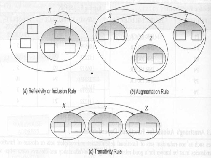
l LET US ASSUME THAT WE ARE GIVEN A TABLE T and THAT ALL SETS OF ATTRIBUTES X, Y, Z ARE CONTAINED IN THE HEADING OF T. THEN FOLLOWING ARE A SET OF INFERENCE RULES, CALLED Armstrong's axioms, TO DERIVE ONE FDS FROM OTHER FDS: RULE 1 Reflexivity(inclusion) IF, Y C X, THEN X Y RULE 2 Augmentation: If X Y, THEN XZ YZ. RULE 3 Transitivity: IF X Y AND Y Z, THEN X Z.

FROM ARMSTRONG'S AXIOMS, A NUMBER OF OTHER RULES OF IMPLICATION AMONG FDS CAN BE PROVED. AGAIN, LET US ASSUME THAT ALL SETS OF ATTRIBUTES W, X, Y, Z ARE CONTAINED IN THE HEADING OF A TABLE T.

• THEN THE FOLLOWING ADDITIONAL RULES CAN BE DERIVED FROM ARMSTRONG'S AXIOMS: • • • RULE 4 X X. Self-determination: RULE 5 Pseudo-transitivity: IF X Y AND YW Z, THEN XW Z. RULE 6 Union or additive: IF X Z AND X Y, THEN X YZ.

RULE 7 Decomposition or projective: IF X YZ, THEN X Y AND X Z. RULE 8 Composition: IF X Y AND Z W, THEN XZ YW. RULE 9 SELF accumulation: IF X YZ AND Z W, THEN X YZW.

Redundant Functional Dependencies • A REDUNDANT FD CAN BE DETECTED USING THE FOLLOWING STEPS: Step 1: START WITH A SET OF S OF FUNCTIONAL DEPENDENCIES (FDS). Step 2: REMOVE AN FD F AND CREATE A SET OF FDS S' = S - f.

Step 3: TEST WHETHER F CAN BE DERIVED FROM THE FDS IN S' BY USING THE SET OF ARMSTRONG'S AXIOMS AND DERIVED RULES. Step 4: IF F CAN BE SO DERIVED, IT IS REDUNDANT , AND HENCE S' = S. OTHERWISE REPLACE F INTO S' SO THAT NOW S' = S + f Step 5: REPEAT STEPS 2 TO 4 FOR ALL FDS IN S.

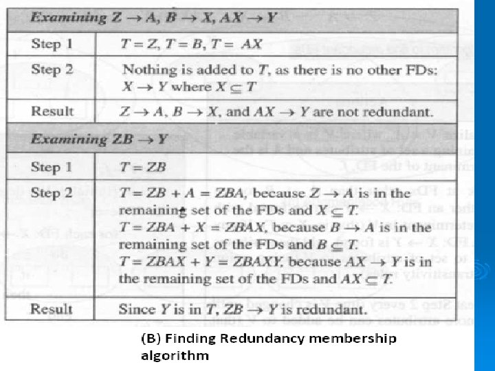
• ARMSTRONG'S AXIOMS AND DERIVED RULES, AS DISCUSSED IN THE PREVIOUS SECTION, CAN BE USED TO FIND REDUNDANT FDS. • FOR EXAMPLE, SUPPOSE THE FOLLOWING SET OF FDS IS GIVEN IN THE ALGORITHM: Z A B X AX Y ZB Y BECAUSE ZB Y Can BE DERIVED FROM OTHER FDS IN THE SET, IT CAN BE

THE FOLLOWING ARGUMENT CAN BE GIVEN: Z A BY AUGMENTATION RULE WILL YIELD ZB AB. B X AND AX Y BY PSEUDOTRANSITIVITY RULE WILL YIELD AB Y. ZB AB AND AB Y by TRANSITIVITY

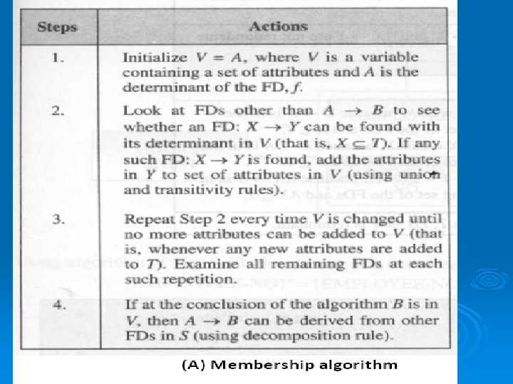
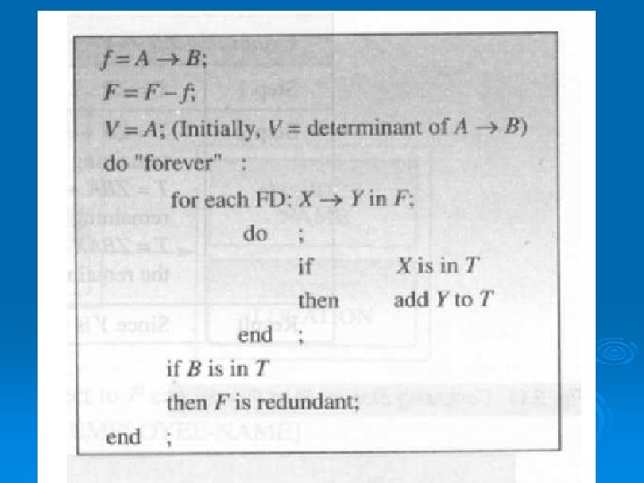
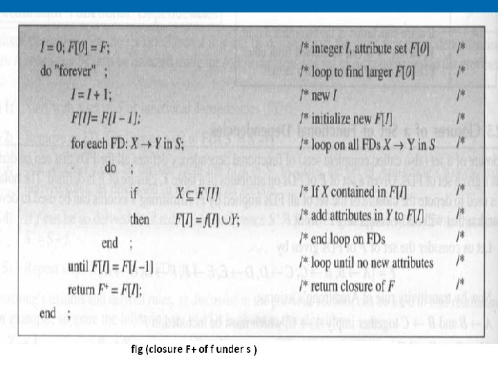
• AN algorithm (CALLED membership algorithm) CAN BE DEVELOPED TO FIND REDUNDANT FDS, THAT IS, TO DETERMINE WHETHER AN FD F(A B) CAN BE DERIVED FROM A SET OF FDS S. FIG. (A) ILLUSTRATES THE STEPS AND THE LOGICS OF THE ALGORITHM. • Using the algorithm of Fig. (A) , following set of FDs can be checked for the redundancy, as shown in Fig. (B). Z A B X AX Y ZB Y

Closures of a Set of Functional Dependencies l l l A closure of a set (also called complete sets) of functional dependency defines all the FDs that can be derived from a given set of FDs. Given a set of FDs on attributes of a table T, closure of F is defined. The notation F+ is used to denote the closure of the set of all FDs implied by F. Armstrong's axioms can be used to develop algorithm that will allow computing F+ from F.

l Let us consider the set of FDs given by F= {A B, B C, C D, D E, E F, F G, G H} Now by transitivity rule of Armstrong's axioms, l l l A B and B C together imply A C, which must be included in F+. Also, B C and C D together imply B D. Every single attribute appearing prior to the terminal one in the sequence ABCDEFGH can be shown by transitivity rule to functionally determine every single attribute on its right in the sequence. Trivial FDs such as A A is also present.

l l Now by union rule of Armstrong's axioms, other FDs can be generated such as A ABCDEFGH. All FDs derived above are contained in F+. FDs have been derived by applying the axioms and rules, an algorithm similar to membership algorithm of Fig. above (b), can be developed. Fig. illustrates such an algorithm to compute a certain subset of the closure. In other words, for a given set F of attributes of table T and a set of S of FDs that hold for T, the set of all attributes of T that are functionally dependent on F, is called closure F+ of F under S.

DECOMPOSITION l l l A functional decomposition is the process of breaking down the functions of an organization into progressively greater (finer and finer) levels of detail. In decomposition, one function is described in greater detail by a set of other supporting functions. In other words, decomposition is done to break the modules in smallest one to convert the data models in normal forms to avoid redundancies.

l l l The decomposition of a relation scheme R consists of replacing the relation schema by two or more relation schemas that each contain a subset of the attributes of R and together include all attributes in R. The algorithm of relational database design starts from a single universal relation schema R= { A 1, A 2, A 3, --, AN }, which includes all the attributes of the database. The universal relation states that every attribute name is unique.

l l Ø Ø Using the functional dependencies, the design algorithms decompose the universal relation schema R into a set of relation schemas D = { R 1, , R 2, R 3, … Rm}. Now, D becomes the relational database schema and D is called a decomposition of R. The decomposition of a relation scheme R= { A 1, A 2, A 3, -----, AN} is its replacement by a set of relation schemes D = { R 1, , R 2, R 3, … Rm} such that R 1 C R for 1 < i < m R 1 U R 2 U R 3 …. U Rm=R.

l l Decomposition helps in eliminating some of the problems of bad design such as redundancy, inconsistencies and anomalies.

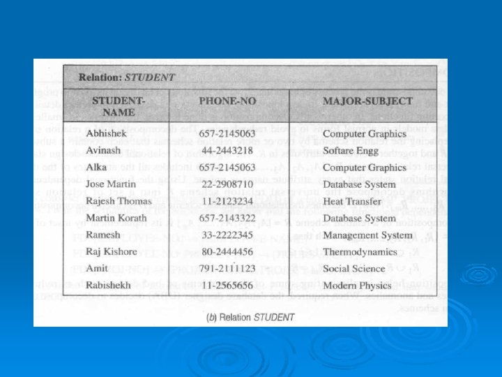
l Let us consider the relation STUDENT_INFO, as shown in Fig. (a). Now, this relation is replaced with the following three relation schemes:

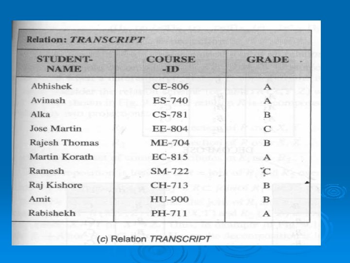
ØThe first relation scheme STUDENT stores only once the phone number and major subject of each student. ØAny change in the phone number will require a change in only one tuple (row) of this relation. The second relation scheme TRANSCRIPT stores the grade of each student in each course in which the student is enrolled. ØThe third relation scheme FACULTY stores the professor of each course that is taught to the students, fig. (b), (c) and (d) illustrates the decomposed relation schemes STUDENT, TRANSCRIPT and FACULTY respectively

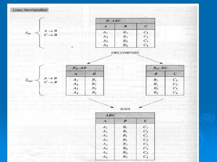
Lossy Decomposition l l l One of the disadvantages of decomposition into two or more relational schemes (or tables) is that some information is lost during retrieval of original relation or table. Let us consider the relation scheme (or table) R (A, B, C) with functional dependencies A B and C B as shown in Fig. The relation R is decomposed into two relations, R 1(A, B) and R 2(B, C).

l l If the two relations R 1 and R 2 are now joined, the join will contain rows in addition to those in R. It can be seen in Fig. that this is not the original table content for R (A, B, C). Since it is difficult to know what table content was started from, information has been lost by the above decomposition and the subsequent pin operation. This phenomenon is known as a lossy decomposition, or lossy-join decomposition.

l l Thus, the decomposition of R(A, B, C) into R 1 and R 2 is lossy when the join of R 1 and R 2 does nor yield the same relation as in R. That means, neither B A nor B C is true. Now, let us consider that relation scheme STUDENT_INFO, as shown in Fig. Above (a) is decomposed into the following two relation schemes: STUDENT (STUDENT-NAME, PHONE-NO, MAJOR-SUBJECT, GRADE) COURSE (COURSE-ID, PROFESSOR)

l The above decomposition is a bad decomposition for the following reasons: • There is redundancy and update anomaly, because the data for the attributes PHONE-NO and MAJORSUBJECT (657 -2145063, Computer Graphics) are repeated. • There is loss of information, because the fact that a student has a given grade in a particular course, is lost.

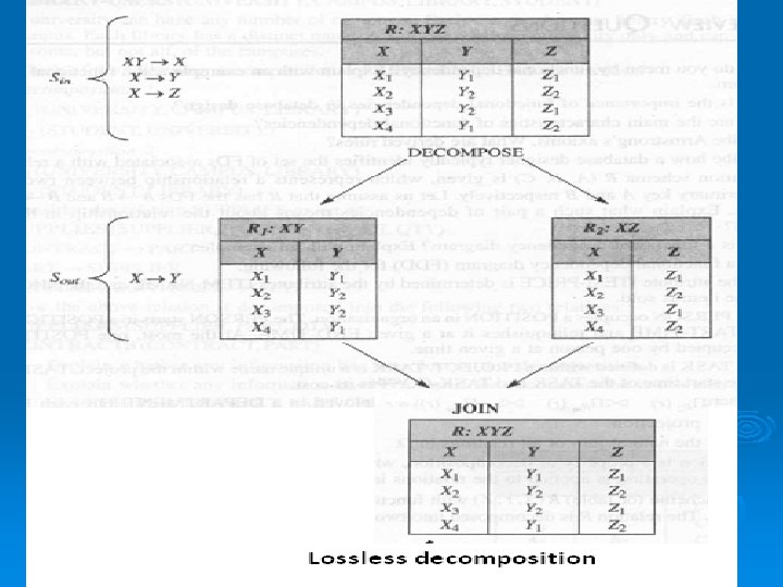
Lossless-Join Decomposition l l l A relational table is decomposed (or factored) into two or more smaller tables, in such a way that the designer can capture the precise content of the original table by joining the decomposed parts. This is called lossless-join (or non-additive join) decomposition. The decomposition of R (X, Y, Z) into R 1(X, Y) and R 2 (X, Z) is lossless if for attributes X, common to both R 1 and R 2, either X Y or Y Z. All decompositions must be lossless.

l l l The word loss in lossless refers to the loss of information. The lossless-join decomposition is always defined with respect to a specific set F of dependencies. A decomposition D={R 1, R 2 , R 3 , …, Rm} of R is said to have the lossless-join property with respect to the set of dependencies F on R if, for every relation state r of R that satisfies F,

The following relation holds:

l Let us consider the relation scheme (or table) R (X, Y, Z) with functional dependencies YZ X, X Y and X Z, as shown in Fig. The relation R is decomposed into two relations, R 1 and R 2 that are defined by following two projections: ØR 1 ØR 2 = projection of R over X, Y = projection of R over X, Z

l l l Where X is the set of common attributes in R 1 and R 2. The decomposition is lossless if R = join of R 1 and R 2 over X And the decomposition is lossy if R C join of R 1 and R 2 over X.

l l l Fig. that the join of R 1 and R 2 yields the same number of rows as does R. The decomposition of R(X, Y, Z) into R 1(X, Y) and R 2(X, Z) is lossless if for attributes X, common to both R 1 and R 2, either X Y or X Z. In Fig. however, the decomposition is lossless because for the common attribute X, both X Y and X Z.

Dependency-Preserving Decomposition l The dependency preservation decomposition is another property of decomposed relational database schema D in which each functional dependency X Y specified in F either appeared directly in one of the relation schemas Ri in the decomposed D or could be inferred from the dependencies that appear in some Ri.

• Decomposition D = { R 1, R 2, R 3, , . . , , Rm} of R is said to be dependency-preserving with respect to F if the union of the projections of F on each Ri, in D is equivalent to F.

l In other words, R C join of R 1, R 1 over X Ø l The dependencies are preserved because each dependency in F represents a constraint on the database. If decomposition is not dependencypreserving, some dependency is lost in the decomposition.