From Transaction Processing to Support for Decision Making

From Transaction Processing to Support for Decision Making CIS 671 Decision Support Systems 1

Computerized Information Systems • Used to “run the business”. • OSU Examples – Personnel & Payroll (ARMS) – Course Offerings – Students, including course enrollments and grades • (estimated $30 M to replace) – Inventory • Transaction Processing Decision Support Systems 2

st 1 Generation DBMS • Designed for Transaction Processing – Hierarchical – IBM – IMS – Network • Management Information Systems – Added later – Mostly standard summary reports • Produced on a regular basis Decision Support Systems 3

Relational DBMS • Codd – particularly designed for “ad hoc” queries • First uses for Transaction Processing • Transaction Data now available on-line – Use it to help Decision Making – Ad Hoc Decision Support Systems 4

Decision Support Systems (DSS) • Use comprehensive view of all aspects of business. – Different business units – Historical data – Summary information • Classes of analysis tools: – Complex “traditional” SQL queries – Many “group-by” and “aggregation” queries (On Line Analytical Processing) – Exploratory data analysis - Data Mining Decision Support Systems 5

Data Warehousing • Properties – Consolidated data from many sources – Spanning long time periods – Augmented with summary information • Size: several gigabytes to terabytes Decision Support Systems 6

Data Warehouse Creation • Integrate schemas from different groups – Semantic mismatches • Different currencies • Different names for same attributes • Different structures for similar tables Decision Support Systems 7

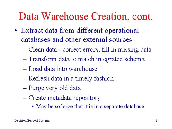
Data Warehouse Creation, cont. • Extract data from different operational databases and other external sources – Clean data - correct errors, fill in missing data – Transform data to match integrated schema – Load data into warehouse – Refresh data in a timely fashion – Purge very old data – Create metadata repository • May be so large that it is in a separate database Decision Support Systems 8

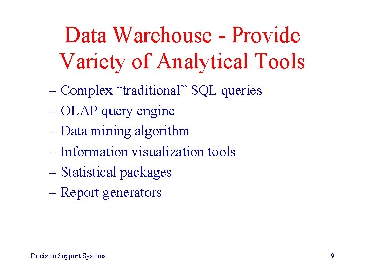
Data Warehouse - Provide Variety of Analytical Tools – Complex “traditional” SQL queries – OLAP query engine – Data mining algorithm – Information visualization tools – Statistical packages – Report generators Decision Support Systems 9

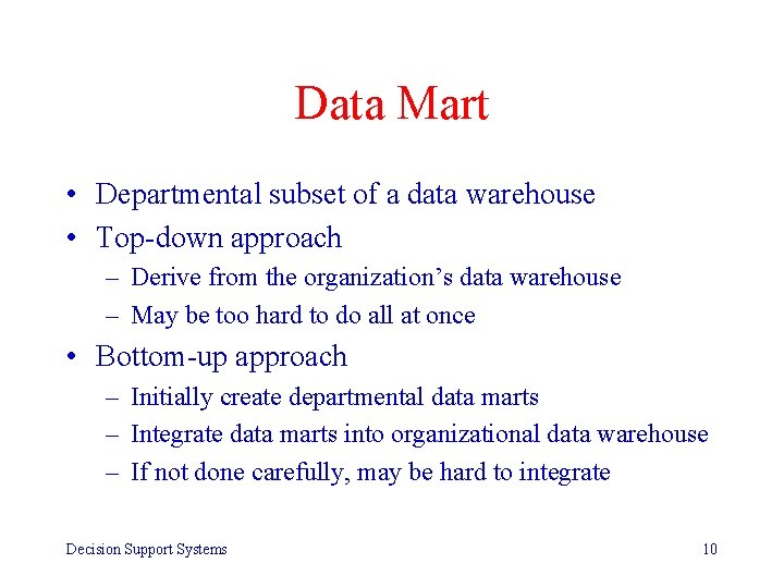
Data Mart • Departmental subset of a data warehouse • Top-down approach – Derive from the organization’s data warehouse – May be too hard to do all at once • Bottom-up approach – Initially create departmental data marts – Integrate data marts into organizational data warehouse – If not done carefully, may be hard to integrate Decision Support Systems 10

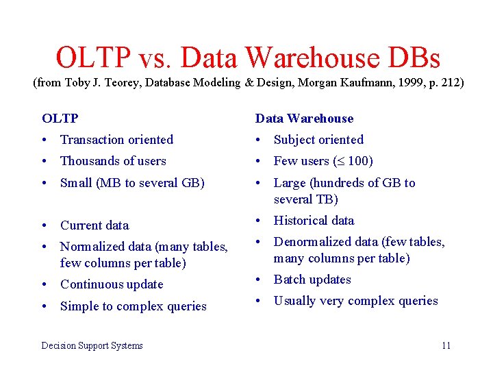
OLTP vs. Data Warehouse DBs (from Toby J. Teorey, Database Modeling & Design, Morgan Kaufmann, 1999, p. 212) OLTP Data Warehouse • Transaction oriented • Subject oriented • Thousands of users • Few users ( 100) • Small (MB to several GB) • Large (hundreds of GB to several TB) • Current data • Historical data • Normalized data (many tables, few columns per table) • Denormalized data (few tables, many columns per table) • Continuous update • Batch updates • Simple to complex queries • Usually very complex queries Decision Support Systems 11

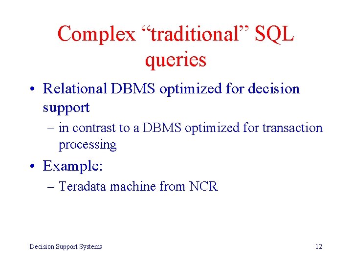
Complex “traditional” SQL queries • Relational DBMS optimized for decision support – in contrast to a DBMS optimized for transaction processing • Example: – Teradata machine from NCR Decision Support Systems 12

On Line Analytical Processing (OLAP) Multidimensional Databases (MDD) Decision Support Systems 13

Example from Finkelstein [Fink 95]: • Note that Branch, Prod. ID, Date Sales, Returns • Note the multidimensionality of the SALES_INFO table. Decision Support Systems 14

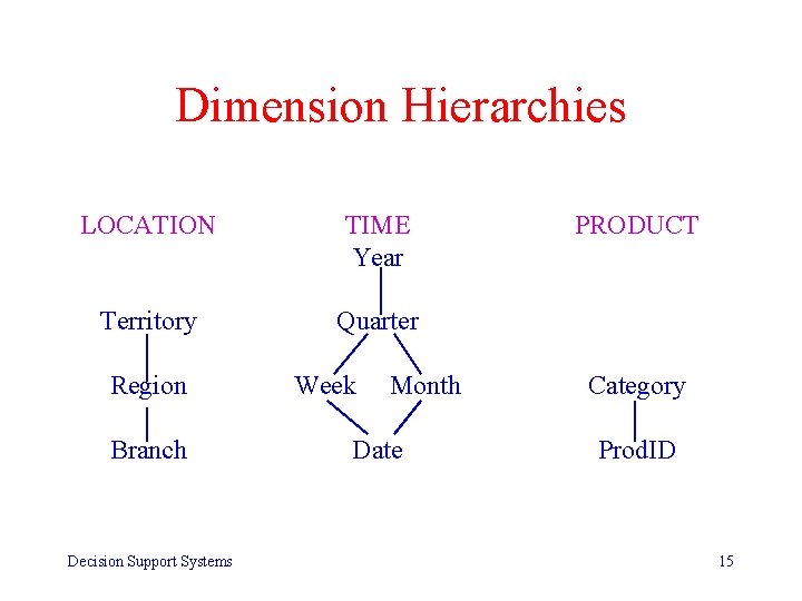
Dimension Hierarchies LOCATION TIME Year Territory Quarter Region Branch Decision Support Systems Week Month Date PRODUCT Category Prod. ID 15

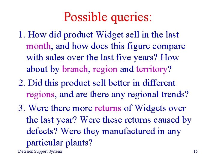
Possible queries: 1. How did product Widget sell in the last month, and how does this figure compare with sales over the last five years? How about by branch, region and territory? 2. Did this product sell better in different regions, and are there any regional trends? 3. Were there more returns of Widgets over the last year? Were these returns caused by defects? Were they manufactured in any particular plants? Decision Support Systems 16

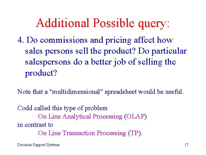
Additional Possible query: 4. Do commissions and pricing affect how sales persons sell the product? Do particular salespersons do a better job of selling the product? Note that a "multidimensional" spreadsheet would be useful. Codd called this type of problem On Line Analytical Processing (OLAP) in contrast to On Line Transaction Processing (TP). Decision Support Systems 17

Codd's rules for OLAP: [Codd 93] 1. Multi-Dimensional Concept View The user should be able to see the data as being multidimensional insofar as it should be easy to 'pivot' or 'slice and dice’. (See later. ) 2. Transparency The OLAP functionality should be provided behind the user's existing software without adversely affecting the functionality of the 'host'. 3. Accessibility OLAP should allow the user to access diverse data stores but see the data within a common 'schema' provided by the OLAP tool. Decision Support Systems 18

OLAP Rules, cont. 4. Consistent Reporting Performance There should not be significant degradation in performance with large numbers of dimensions or large quantities of data. 5. Client-Server Architecture Since much of the data is on mainframes, and the users work on PCs, the OLAP tool must be able to bring the two together! 6. Generic Dimensionality Data dimensions must all be treated equally. Functions available for one dimension must be available for others. Decision Support Systems 19

OLAP Rules, cont. 7. Dynamic Sparse Matrix Handling The OLAP tool should be able to work out for itself the most efficient way to store sparse matrix data. 8. Multi User Support This is self-evident. 9. Unrestricted Cross-Dimensional Operations e. g. , individual office overheads are allocated according to total corporate overheads divided in proportion to individual office sales. Decision Support Systems 20

OLAP Rules, cont. 10. Intuitive Data Manipulation Navigation should be done by operations on individual cells rather than menus. 11. Flexible Reporting Row and column headings must be capable of more than one dimension each, and of displaying subsets of any dimension. 12. Unlimited Dimensions and Aggregation Levels At least 15 dimensions may be required, and within each there may be many hierarchical levels. Decision Support Systems 21

Example from Finkelstein [Fink 95]: • Note that Branch, Prod. ID, Date Sales, Returns • Note the multidimensionality of the SALES_INFO table. Decision Support Systems 22

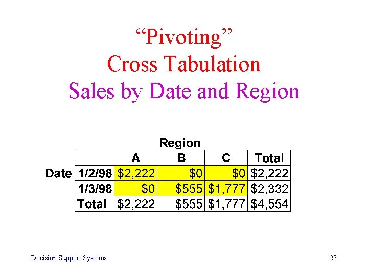
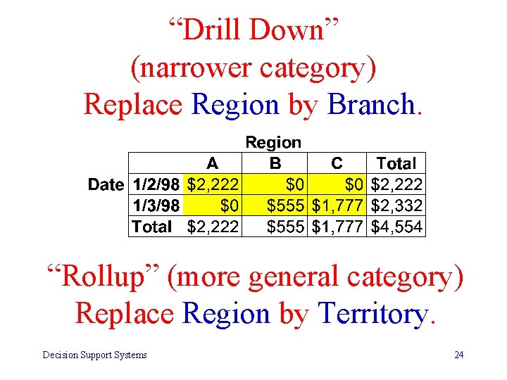
“Pivoting” Cross Tabulation Sales by Date and Region Decision Support Systems 23

“Drill Down” (narrower category) Replace Region by Branch. “Rollup” (more general category) Replace Region by Territory. Decision Support Systems 24

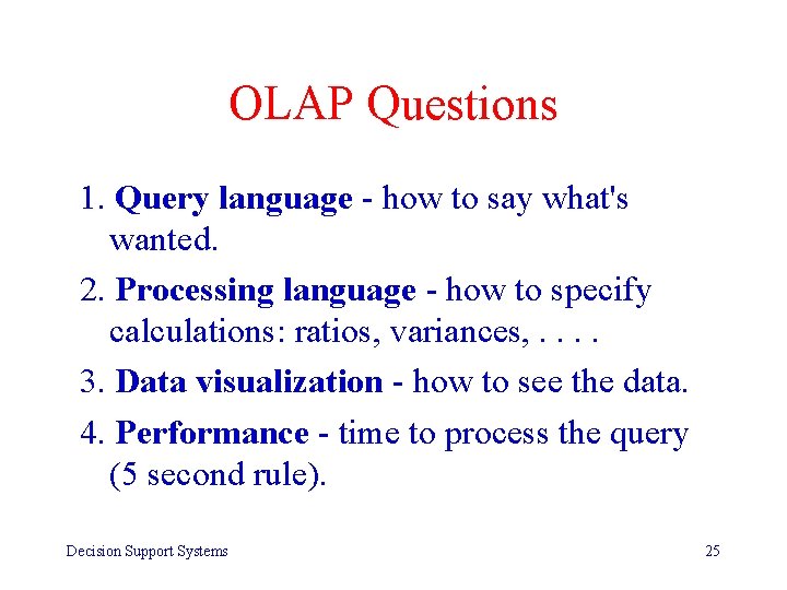
OLAP Questions 1. Query language - how to say what's wanted. 2. Processing language - how to specify calculations: ratios, variances, . . 3. Data visualization - how to see the data. 4. Performance - time to process the query (5 second rule). Decision Support Systems 25

OLAP References [Codd 93] E. F. Codd, S. B. Codd, and C. T. Salley, "Providing OLAP to User Analysts: An IT Mandate, " Codd & Date Inc. , 1993. [Fink 95] Richard Finkelstein, "MDD: Database Reaches the Next Dimension, " DATABASE Programming and Design, 8(4), April 1995. Decision Support Systems 26

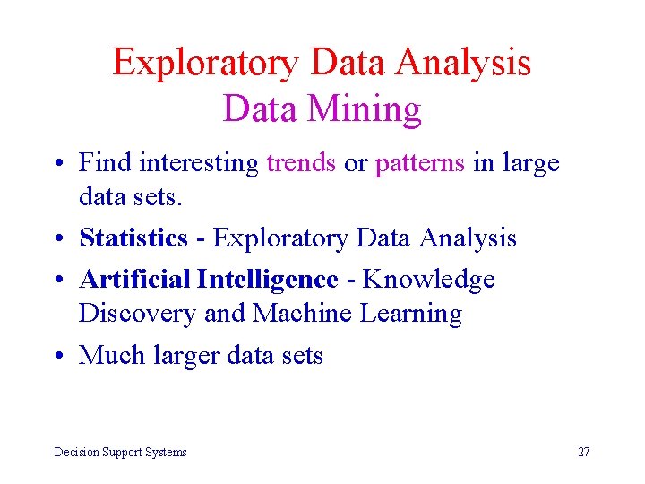
Exploratory Data Analysis Data Mining • Find interesting trends or patterns in large data sets. • Statistics - Exploratory Data Analysis • Artificial Intelligence - Knowledge Discovery and Machine Learning • Much larger data sets Decision Support Systems 27

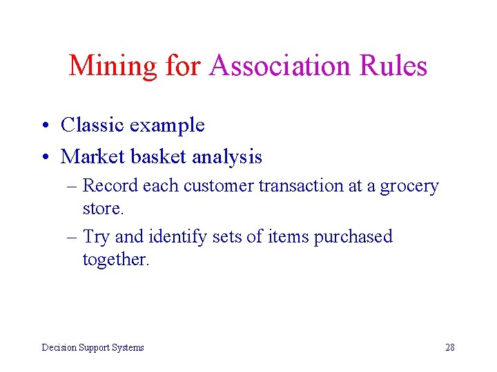
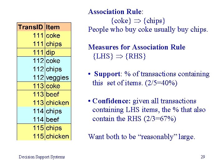
Mining for Association Rules • Classic example • Market basket analysis – Record each customer transaction at a grocery store. – Try and identify sets of items purchased together. Decision Support Systems 28

Association Rule: {coke} {chips} People who buy coke usually buy chips. Measures for Association Rule {LHS} {RHS} • Support: % of transactions containing this set of items. (2/5=40%) • Confidence: given all transactions containing LHS items, the % that also contain the RHS (2/3=67%) Want both to be “reasonably” large. Decision Support Systems 29

On-Line Analytical Processing (OLAP) Part II: CIS 671 Elmasri & Navathe § 26. 1 Decision Support Systems 30

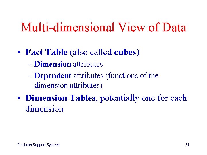
Multi-dimensional View of Data • Fact Table (also called cubes) – Dimension attributes – Dependent attributes (functions of the dimension attributes) • Dimension Tables, potentially one for each dimension Decision Support Systems 31

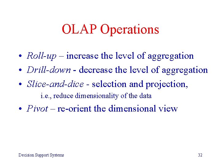
OLAP Operations • Roll-up – increase the level of aggregation • Drill-down - decrease the level of aggregation • Slice-and-dice - selection and projection, i. e. , reduce dimensionality of the data • Pivot – re-orient the dimensional view Decision Support Systems 32

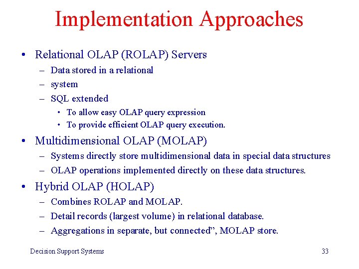
Implementation Approaches • Relational OLAP (ROLAP) Servers – Data stored in a relational – system – SQL extended • To allow easy OLAP query expression • To provide efficient OLAP query execution. • Multidimensional OLAP (MOLAP) – Systems directly store multidimensional data in special data structures – OLAP operations implemented directly on these data structures. • Hybrid OLAP (HOLAP) – Combines ROLAP and MOLAP. – Detail records (largest volume) in relational database. – Aggregations in separate, but connected”, MOLAP store. Decision Support Systems 33

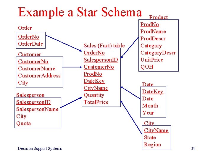
Example a Star Schema Order. No Order. Date Customer. No Customer. Name Customer. Address City Salesperson. ID Salesperson. Name City Quota Decision Support Systems Sales (Fact) table Order. No Salesperson. ID Customer. No Prod. No Date. Key City. Name Quantity Total. Price Product Prod. No Prod. Name Prod. Descr Category. Descr Unit. Price QOH Date. Key Date Month Year City. Name State Region 34

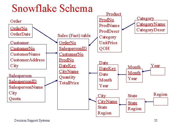
Snowflake Schema Order. No Order. Date Customer. No Customer. Name Customer. Address City Salesperson. ID Salesperson. Name City Quota Decision Support Systems Sales (Fact) table Order. No Salesperson. ID Customer. No Prod. No Date. Key City. Name Quantity Total. Price Product Prod. No Prod. Name Prod. Descr Category Unit. Price QOH Category. Name Category. Descr Date. Key Date Month Year City. Name State Region Year Region 35

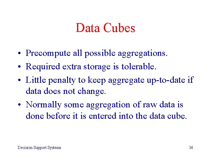
Data Cubes • Precompute all possible aggregations. • Required extra storage is tolerable. • Little penalty to keep aggregate up-to-date if data does not change. • Normally some aggregation of raw data is done before it is entered into the data cube. Decision Support Systems 36

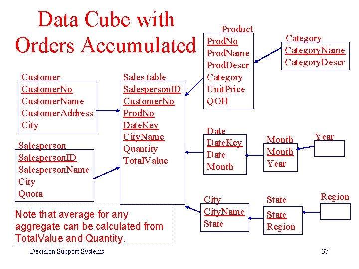
Data Cube with Orders Accumulated Customer. No Customer. Name Customer. Address City Salesperson. ID Salesperson. Name City Quota Sales table Salesperson. ID Customer. No Prod. No Date. Key City. Name Quantity Total. Value Note that average for any aggregate can be calculated from Total. Value and Quantity. Decision Support Systems Product Prod. No Prod. Name Prod. Descr Category Unit. Price QOH Category. Name Category. Descr Date. Key Date Month Year City. Name State Region Year Region 37

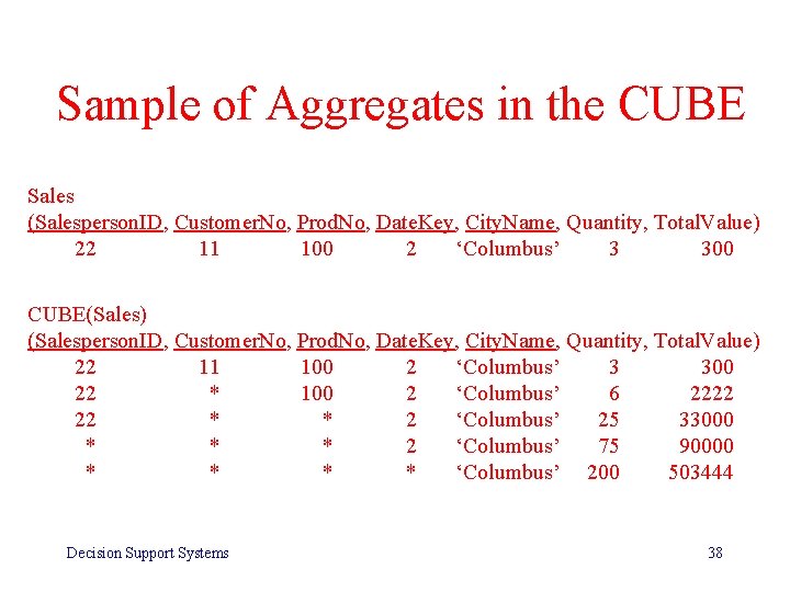
Sample of Aggregates in the CUBE Sales (Salesperson. ID, Customer. No, Prod. No, Date. Key, City. Name, Quantity, Total. Value) 22 11 100 2 ‘Columbus’ 3 300 CUBE(Sales) (Salesperson. ID, Customer. No, Prod. No, Date. Key, City. Name, Quantity, Total. Value) 22 11 100 2 ‘Columbus’ 3 300 22 * 100 2 ‘Columbus’ 6 2222 22 * * 2 ‘Columbus’ 25 33000 * * * 2 ‘Columbus’ 75 90000 * * ‘Columbus’ 200 503444 Decision Support Systems 38

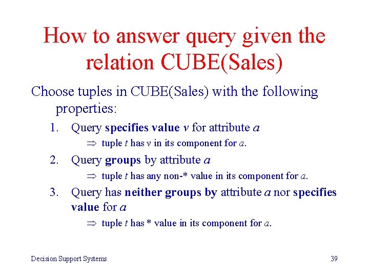
How to answer query given the relation CUBE(Sales) Choose tuples in CUBE(Sales) with the following properties: 1. Query specifies value v for attribute a tuple t has v in its component for a. 2. Query groups by attribute a tuple t has any non-* value in its component for a. 3. Query has neither groups by attribute a nor specifies value for a tuple t has * value in its component for a. Decision Support Systems 39

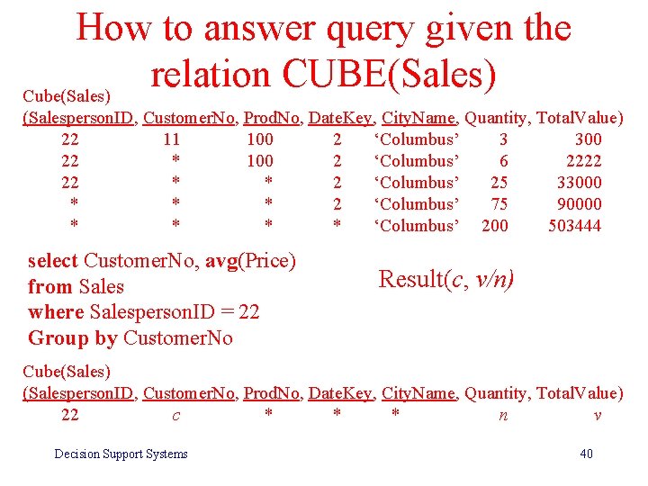
How to answer query given the relation CUBE(Sales) Cube(Sales) (Salesperson. ID, Customer. No, Prod. No, Date. Key, City. Name, Quantity, Total. Value) 22 11 100 2 ‘Columbus’ 3 300 22 * 100 2 ‘Columbus’ 6 2222 22 * * 2 ‘Columbus’ 25 33000 * * * 2 ‘Columbus’ 75 90000 * * ‘Columbus’ 200 503444 select Customer. No, avg(Price) from Sales where Salesperson. ID = 22 Group by Customer. No Result(c, v/n) Cube(Sales) (Salesperson. ID, Customer. No, Prod. No, Date. Key, City. Name, Quantity, Total. Value) 22 c * * * n v Decision Support Systems 40

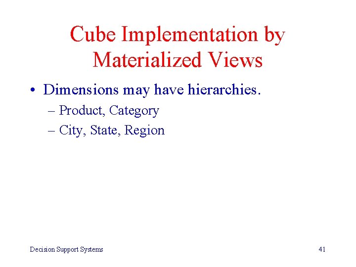
Cube Implementation by Materialized Views • Dimensions may have hierarchies. – Product, Category – City, State, Region Decision Support Systems 41

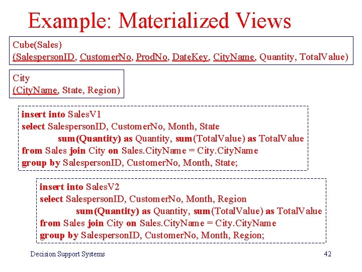
Example: Materialized Views Cube(Sales) (Salesperson. ID, Customer. No, Prod. No, Date. Key, City. Name, Quantity, Total. Value) City (City. Name, State, Region) insert into Sales. V 1 select Salesperson. ID, Customer. No, Month, State sum(Quantity) as Quantity, sum(Total. Value) as Total. Value from Sales join City on Sales. City. Name = City. Name group by Salesperson. ID, Customer. No, Month, State; insert into Sales. V 2 select Salesperson. ID, Customer. No, Month, Region sum(Quantity) as Quantity, sum(Total. Value) as Total. Value from Sales join City on Sales. City. Name = City. Name group by Salesperson. ID, Customer. No, Month, Region; Decision Support Systems 42

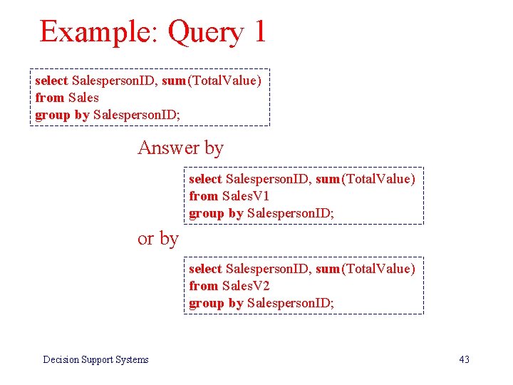
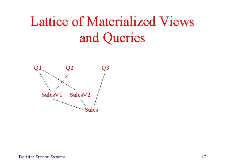
Example: Query 1 select Salesperson. ID, sum(Total. Value) from Sales group by Salesperson. ID; Answer by select Salesperson. ID, sum(Total. Value) from Sales. V 1 group by Salesperson. ID; or by select Salesperson. ID, sum(Total. Value) from Sales. V 2 group by Salesperson. ID; Decision Support Systems 43

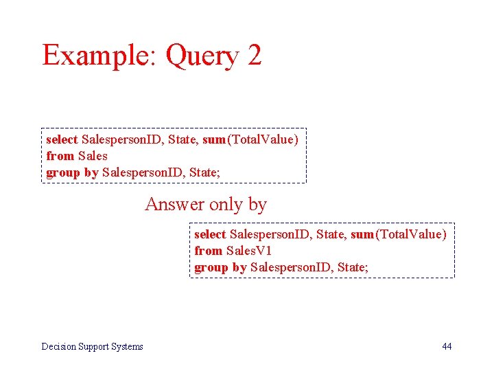
Example: Query 2 select Salesperson. ID, State, sum(Total. Value) from Sales group by Salesperson. ID, State; Answer only by select Salesperson. ID, State, sum(Total. Value) from Sales. V 1 group by Salesperson. ID, State; Decision Support Systems 44

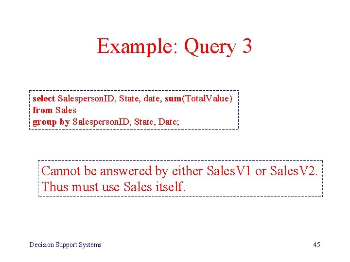
Example: Query 3 select Salesperson. ID, State, date, sum(Total. Value) from Sales group by Salesperson. ID, State, Date; Cannot be answered by either Sales. V 1 or Sales. V 2. Thus must use Sales itself. Decision Support Systems 45

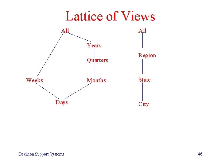
Lattice of Views All Years Quarters Weeks Months Days Decision Support Systems Region State City 46

Lattice of Materialized Views and Queries Q 1 Sales. V 1 Q 2 Q 3 Sales. V 2 Sales Decision Support Systems 47

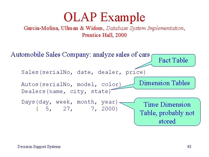
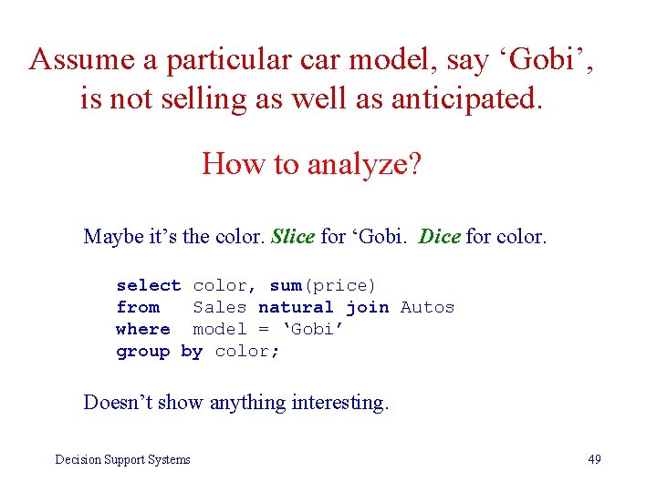
OLAP Example Garcia-Molina, Ullman & Widom, Database System Implementation, Prentice Hall, 2000 Automobile Sales Company: analyze sales of cars Fact Table Sales(serial. No, date, dealer, price) Autos(serial. No, model, color) Dealers(name, city, state) Dimension Tables Days(day, week, month, year) ( 5, 27, 7, 2000) Time Dimension Table, probably not stored Decision Support Systems 48

Assume a particular car model, say ‘Gobi’, is not selling as well as anticipated. How to analyze? Maybe it’s the color. Slice for ‘Gobi. Dice for color. select color, sum(price) from Sales natural join Autos where model = ‘Gobi’ group by color; Doesn’t show anything interesting. Decision Support Systems 49

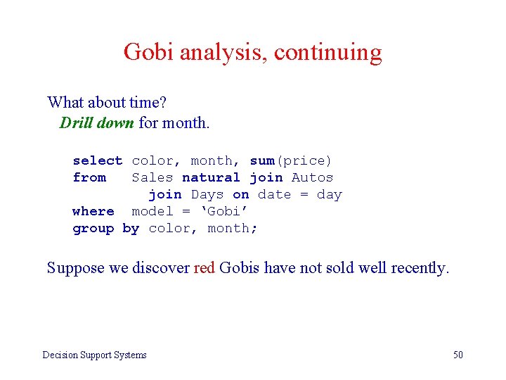
Gobi analysis, continuing What about time? Drill down for month. select color, month, sum(price) from Sales natural join Autos join Days on date = day where model = ‘Gobi’ group by color, month; Suppose we discover red Gobis have not sold well recently. Decision Support Systems 50

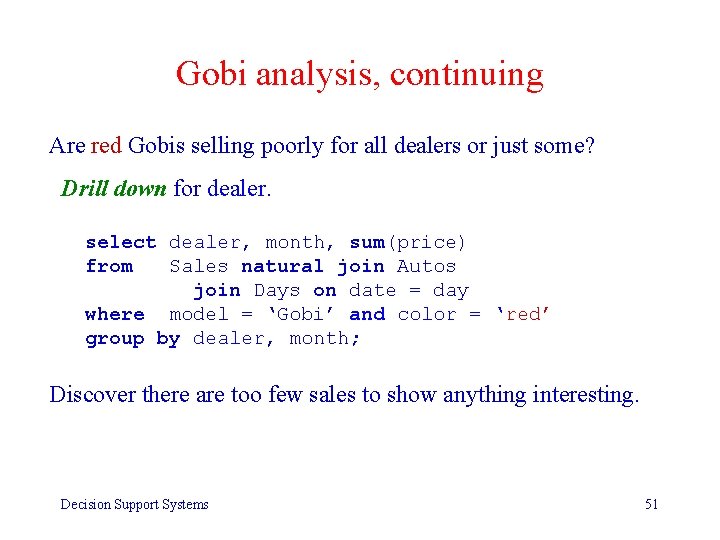
Gobi analysis, continuing Are red Gobis selling poorly for all dealers or just some? Drill down for dealer. select dealer, month, sum(price) from Sales natural join Autos join Days on date = day where model = ‘Gobi’ and color = ‘red’ group by dealer, month; Discover there are too few sales to show anything interesting. Decision Support Systems 51

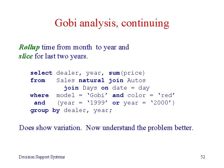
Gobi analysis, continuing Rollup time from month to year and slice for last two years. select dealer, year, sum(price) from Sales natural join Autos join Days on date = day where model = ‘Gobi’ and color = ‘red’ and (year = ‘ 1999’ or year = ‘ 2000’) group by dealer, year; Does show variation. Now understand the problem better. Decision Support Systems 52

Administration • • Lab assignments and HWs posted on the web. Clarifications/Questions? Please use appropriate online submit command Teams of 2 allowed but make contribution of each team member explicit especially in the lab assignment. • Extra Credit assignment in lab. • Bring questions to class on Thursday Decision Support Systems 53

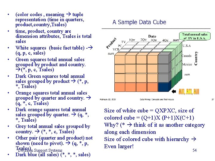
• • • (color codes , meaning tuple representation (time in quarters, product, country, Tsales) time, product, country are dimension attributes, Tsales is total sales White squares (basic fact table) - (q, p, c, sales) Green squares total annual sales grouped by product and country. (*, p, c, Tsales) Dark Green squares total annual sales grouped by product (*, p, *, Tsales) Orange squares total annual sales grouped by quarter and country. (q, *, c, Tsales) Dark orange squares total annual sales grouped by quarter. (q, *, *, Tsales) Grey total annual sales grouped by country. (*, *, c, Tsales) Other pair (quarter and product) not shown (need to pivot). (q, *, p, Tsales) Decision Support Systems Dark blue (all sales) (*, *, *, sales) Size of white cube = QXPXC, size of colored cube = (Q+1)X (P+1)X(C+1) Why? (* think of it as another category along each dimension Size of colored cube with hierarchy Even larger! 54

Decision Support Systems 55

Aggregation causes Database Explosion in Large Multi-dimensional Applications as the Number of Dimensions Increases Based on Nigel Pendse, “Database Explosion”, www. olapreport. com/Database. Explosion. htm Decision Support Systems 56

Factors not causing data explosion • Poor handling of data sparsity. – No more than factor of 4 vs. factors of 10 s or 100 s • Type of database technology. – Although optimized storage technology will be significantly better. • Lack of data compression. – Compression is helpful, but explosion still occurs. • Software errors – Again, a different problem. Decision Support Systems 57

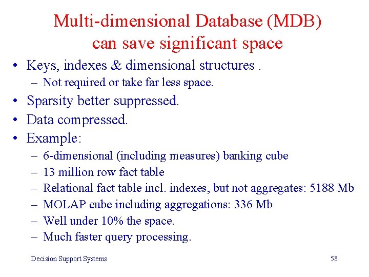
Multi-dimensional Database (MDB) can save significant space • Keys, indexes & dimensional structures. – Not required or take far less space. • Sparsity better suppressed. • Data compressed. • Example: – – – 6 -dimensional (including measures) banking cube 13 million row fact table Relational fact table incl. indexes, but not aggregates: 5188 Mb MOLAP cube including aggregations: 336 Mb Well under 10% the space. Much faster query processing. Decision Support Systems 58

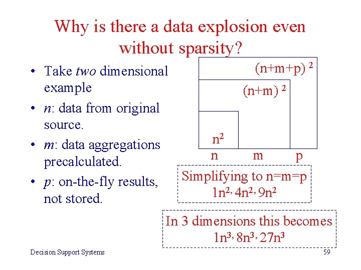
Why is there a data explosion even without sparsity? (n+m+p) 2 • Take two dimensional example (n+m) 2 • n: data from original source. 2 n • m: data aggregations n m p precalculated. Simplifying to n=m=p • p: on-the-fly results, 2, 4 n 2, 9 n 2 1 n not stored. In 3 dimensions this becomes 1 n 3, 8 n 3, 27 n 3 Decision Support Systems 59

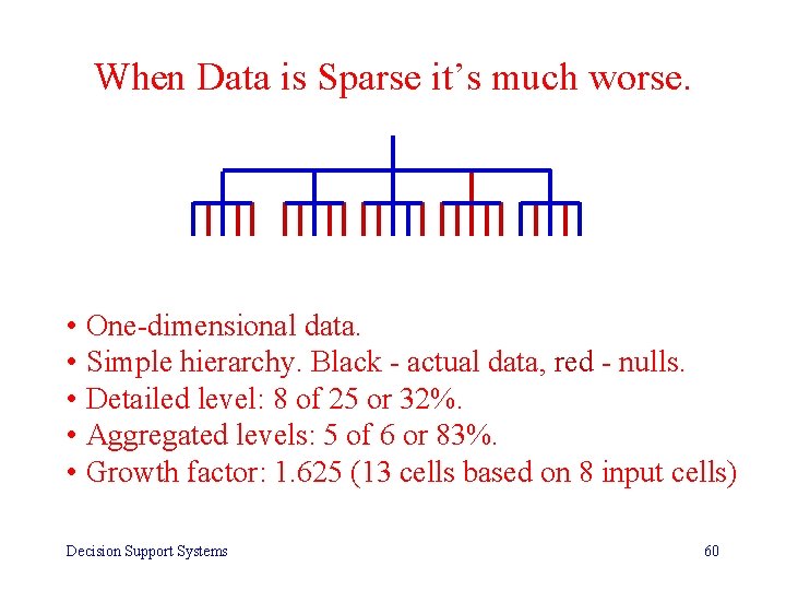
When Data is Sparse it’s much worse. • One-dimensional data. • Simple hierarchy. Black - actual data, red - nulls. • Detailed level: 8 of 25 or 32%. • Aggregated levels: 5 of 6 or 83%. • Growth factor: 1. 625 (13 cells based on 8 input cells) Decision Support Systems 60

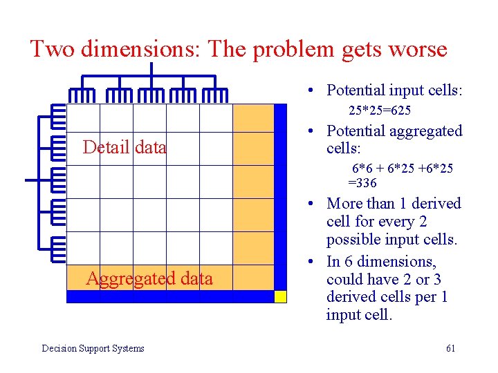
Two dimensions: The problem gets worse • Potential input cells: 25*25=625 Detail data • Potential aggregated cells: 6*6 + 6*25 +6*25 =336 Aggregated data Decision Support Systems • More than 1 derived cell for every 2 possible input cells. • In 6 dimensions, could have 2 or 3 derived cells per 1 input cell. 61

What about higher dimensions? • • • One percent density, 6 of 625 input cells. Yields 29 computed cells. I. e. , 35 total cells, only 6 input. Growth factor: 5. 83. Growth factor per dimension: sqrt(5. 83)=2. 4. – Called compound growth factor (CGF). • CGF is typically in the range 1. 5 to 2. 5. • CGF increases as sparsity increases. • With large dimensions, will often be more consolidation. – (Many thousands of products more levels of groupings. ) • With CGF of 2. 0, extra dimension with no increase in input data, will double size of fully computed database. Decision Support Systems 62

So what is the problem? • Disk space increases. • Can software handle this much data? • Time to load and update database increases. – Could take days to load the database. Decision Support Systems 63

What to do? • Avoid fully pre-calculating any multidimensional object with more than 5 sparse dimensions. • Reduce sparsity of individual data objects: – Use good application design. What to pre-calculate? • Data that is slow to calculate at run-time because it depends on many other cells or complex formulae. • Data that is frequently viewed. • Data that is the basis of many other calculations. • Note: If too much is precalculated, performance may decrease because cache will not include as much useful data. Decision Support Systems 64