From financial options to real options 2 Financial

From financial options to real options 2. Financial options Prof. André Farber Solvay Business School Hanoi April 13, 2000 Financial options 1

Definitions • A call (put) contract gives to the owner – the right : – to buy (sell) – an underlying asset (stocks, bonds, portfolios, . . ) – on or before some future date (maturity) • on : "European" option • before: "American" option • at a price set in advance (the exercise price or striking price) • Buyer pays a premium to the seller (writer) Financial options 2

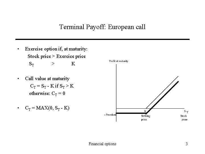
Terminal Payoff: European call • Exercise option if, at maturity: Stock price > Exercice price ST > K • Call value at maturity CT = ST - K if ST > K otherwise: CT = 0 • CT = MAX(0, ST - K) Financial options 3

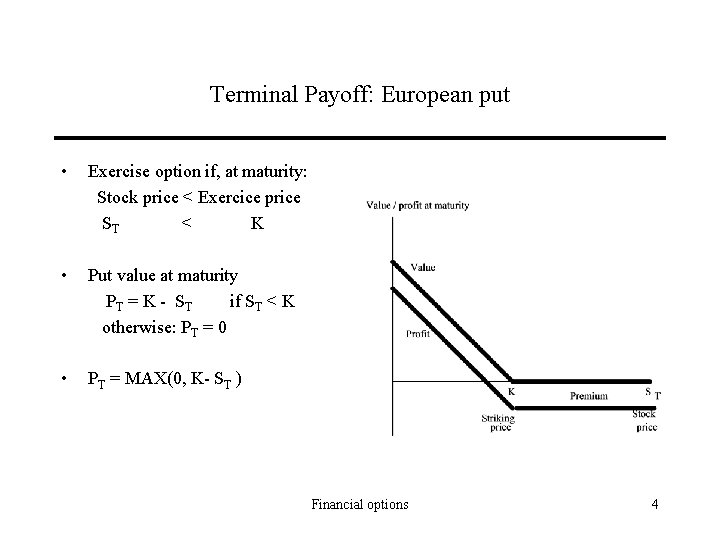
Terminal Payoff: European put • Exercise option if, at maturity: Stock price < Exercice price ST < K • Put value at maturity PT = K - S T if ST < K otherwise: PT = 0 • PT = MAX(0, K- ST ) Financial options 4

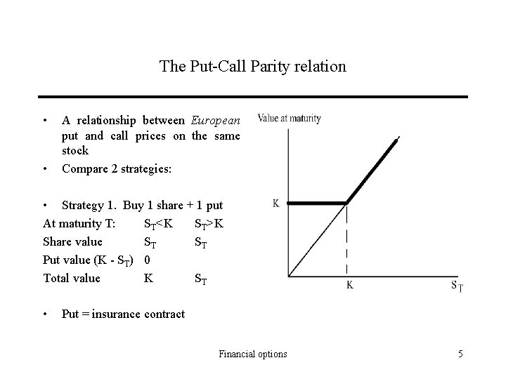
The Put-Call Parity relation • • A relationship between European put and call prices on the same stock Compare 2 strategies: • Strategy 1. Buy 1 share + 1 put At maturity T: ST<K ST>K Share value ST ST Put value (K - ST) 0 Total value K ST • Put = insurance contract Financial options 5

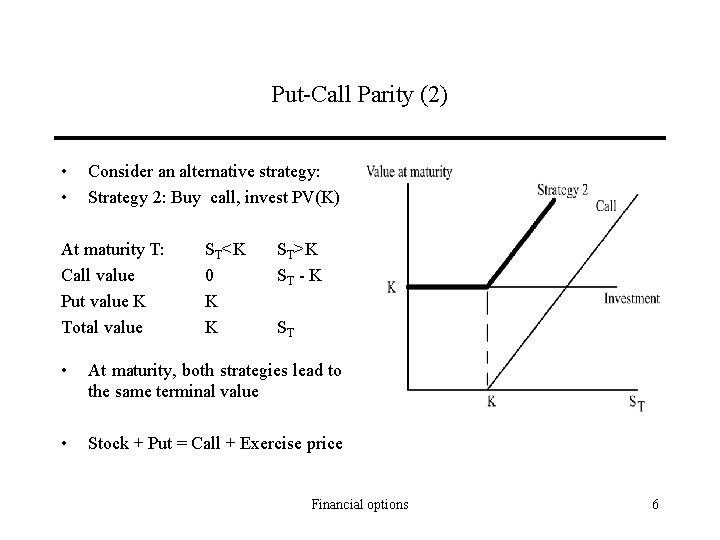
Put-Call Parity (2) • • Consider an alternative strategy: Strategy 2: Buy call, invest PV(K) At maturity T: Call value Put value K Total value ST<K 0 K K ST>K ST - K ST • At maturity, both strategies lead to the same terminal value • Stock + Put = Call + Exercise price Financial options 6

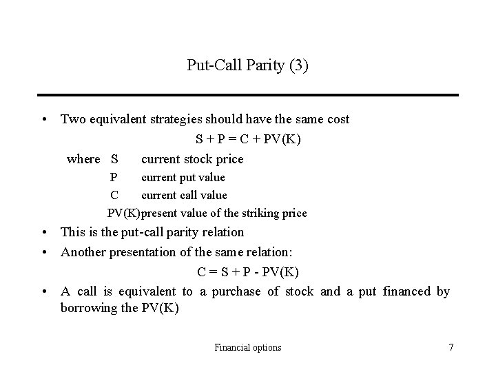
Put-Call Parity (3) • Two equivalent strategies should have the same cost S + P = C + PV(K) where S current stock price P current put value C current call value PV(K)present value of the striking price • This is the put-call parity relation • Another presentation of the same relation: C = S + P - PV(K) • A call is equivalent to a purchase of stock and a put financed by borrowing the PV(K) Financial options 7

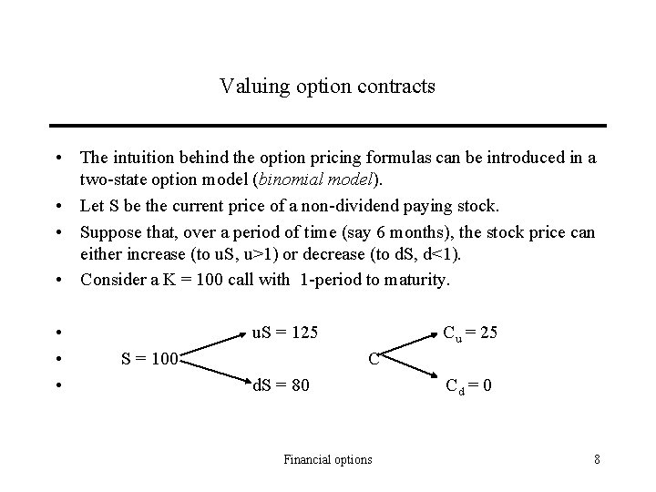
Valuing option contracts • The intuition behind the option pricing formulas can be introduced in a two-state option model (binomial model). • Let S be the current price of a non-dividend paying stock. • Suppose that, over a period of time (say 6 months), the stock price can either increase (to u. S, u>1) or decrease (to d. S, d<1). • Consider a K = 100 call with 1 -period to maturity. • • • u. S = 125 S = 100 Cu = 25 C d. S = 80 Financial options Cd = 0 8

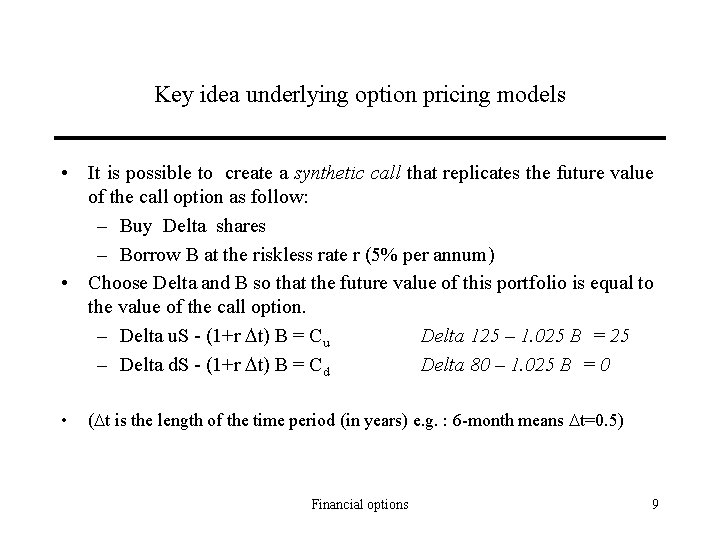
Key idea underlying option pricing models • It is possible to create a synthetic call that replicates the future value of the call option as follow: – Buy Delta shares – Borrow B at the riskless rate r (5% per annum) • Choose Delta and B so that the future value of this portfolio is equal to the value of the call option. – Delta u. S - (1+r t) B = Cu Delta 125 – 1. 025 B = 25 – Delta d. S - (1+r t) B = Cd Delta 80 – 1. 025 B = 0 • ( t is the length of the time period (in years) e. g. : 6 -month means t=0. 5) Financial options 9

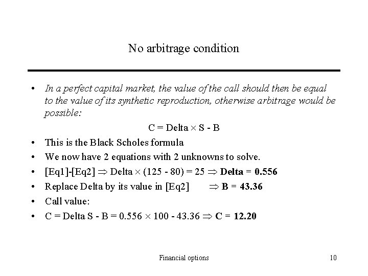
No arbitrage condition • In a perfect capital market, the value of the call should then be equal to the value of its synthetic reproduction, otherwise arbitrage would be possible: C = Delta S - B • This is the Black Scholes formula • We now have 2 equations with 2 unknowns to solve. • Eq 1 - Eq 2 Delta (125 - 80) = 25 Delta = 0. 556 • Replace Delta by its value in Eq 2 B = 43. 36 • Call value: • C = Delta S - B = 0. 556 100 - 43. 36 C = 12. 20 Financial options 10

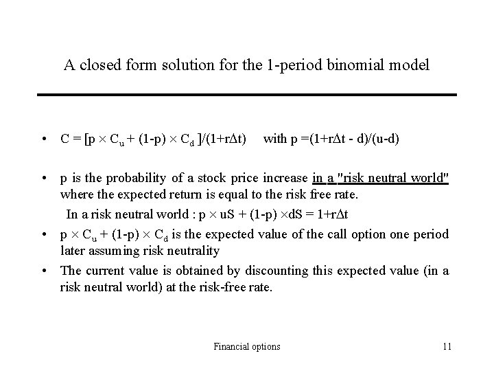
A closed form solution for the 1 -period binomial model • C = [p Cu + (1 -p) Cd ]/(1+r t) with p =(1+r t - d)/(u-d) • p is the probability of a stock price increase in a "risk neutral world" where the expected return is equal to the risk free rate. In a risk neutral world : p u. S + (1 -p) d. S = 1+r t • p Cu + (1 -p) Cd is the expected value of the call option one period later assuming risk neutrality • The current value is obtained by discounting this expected value (in a risk neutral world) at the risk-free rate. Financial options 11

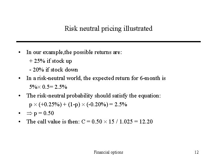
Risk neutral pricing illustrated • In our example, the possible returns are: + 25% if stock up - 20% if stock down • In a risk-neutral world, the expected return for 6 -month is 5% 0. 5= 2. 5% • The risk-neutral probability should satisfy the equation: p (+0. 25%) + (1 -p) (-0. 20%) = 2. 5% • p = 0. 50 • The call value is then: C = 0. 50 15 / 1. 025 = 12. 20 Financial options 12

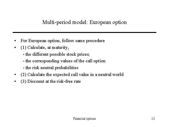
Multi-period model: European option • For European option, follow same procedure • (1) Calculate, at maturity, - the different possible stock prices; - the corresponding values of the call option - the risk neutral probabilities • (2) Calculate the expected call value in a neutral world • (3) Discount at the risk-free rate Financial options 13

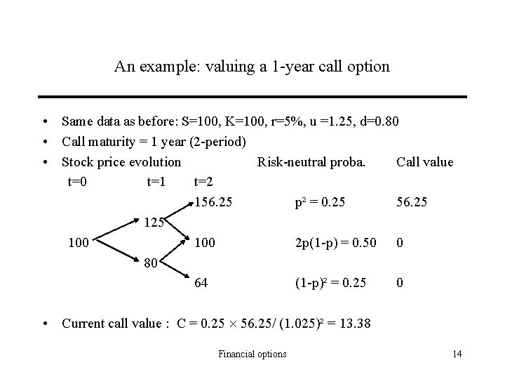
An example: valuing a 1 -year call option • Same data as before: S=100, K=100, r=5%, u =1. 25, d=0. 80 • Call maturity = 1 year (2 -period) • Stock price evolution Risk-neutral proba. Call value t=0 t=1 t=2 156. 25 p² = 0. 25 56. 25 100 100 2 p(1 -p) = 0. 50 0 80 64 (1 -p)² = 0. 25 0 • Current call value : C = 0. 25 56. 25/ (1. 025)² = 13. 38 Financial options 14

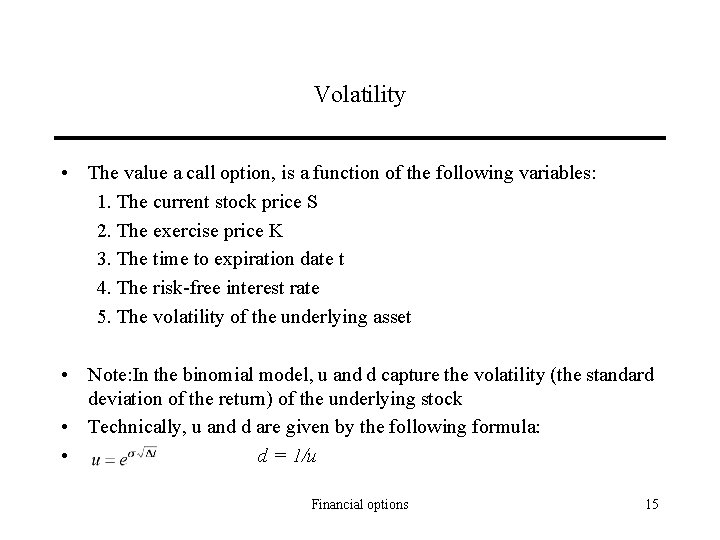
Volatility • The value a call option, is a function of the following variables: 1. The current stock price S 2. The exercise price K 3. The time to expiration date t 4. The risk-free interest rate 5. The volatility of the underlying asset • Note: In the binomial model, u and d capture the volatility (the standard deviation of the return) of the underlying stock • Technically, u and d are given by the following formula: • d = 1/u Financial options 15

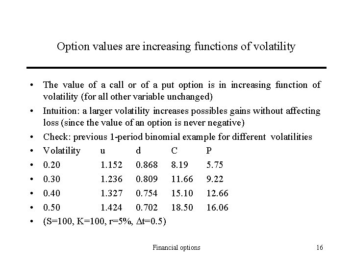
Option values are increasing functions of volatility • The value of a call or of a put option is in increasing function of volatility (for all other variable unchanged) • Intuition: a larger volatility increases possibles gains without affecting loss (since the value of an option is never negative) • Check: previous 1 -period binomial example for different volatilities • Volatility u d C P • 0. 20 1. 152 0. 868 8. 19 5. 75 • 0. 30 1. 236 0. 809 11. 66 9. 22 • 0. 40 1. 327 0. 754 15. 10 12. 66 • 0. 50 1. 424 0. 702 18. 50 16. 06 • (S=100, K=100, r=5%, t=0. 5) Financial options 16

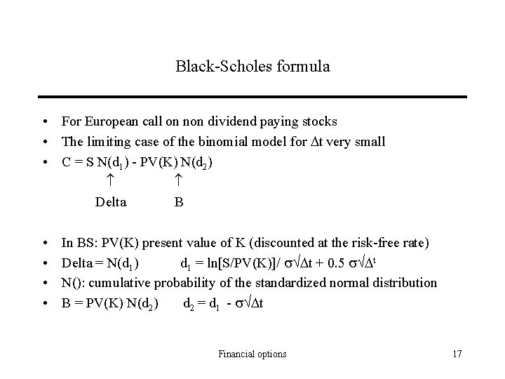
Black-Scholes formula • For European call on non dividend paying stocks • The limiting case of the binomial model for t very small • C = S N(d 1) - PV(K) N(d 2) Delta B • • In BS: PV(K) present value of K (discounted at the risk-free rate) Delta = N(d 1) d 1 = ln[S/PV(K)]/ t + 0. 5 t N(): cumulative probability of the standardized normal distribution B = PV(K) N(d 2) d 2 = d 1 - t Financial options 17

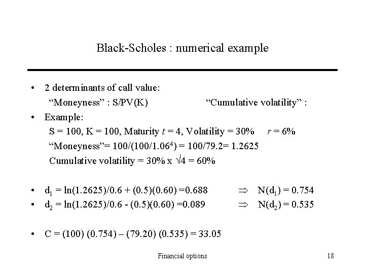
Black-Scholes : numerical example • 2 determinants of call value: “Moneyness” : S/PV(K) “Cumulative volatility” : • Example: S = 100, K = 100, Maturity t = 4, Volatility = 30% r = 6% “Moneyness”= 100/(100/1. 064) = 100/79. 2= 1. 2625 Cumulative volatility = 30% x 4 = 60% • d 1 = ln(1. 2625)/0. 6 + (0. 5)(0. 60) =0. 688 • d 2 = ln(1. 2625)/0. 6 - (0. 5)(0. 60) =0. 089 N(d 1) = 0. 754 N(d 2) = 0. 535 • C = (100) (0. 754) – (79. 20) (0. 535) = 33. 05 Financial options 18

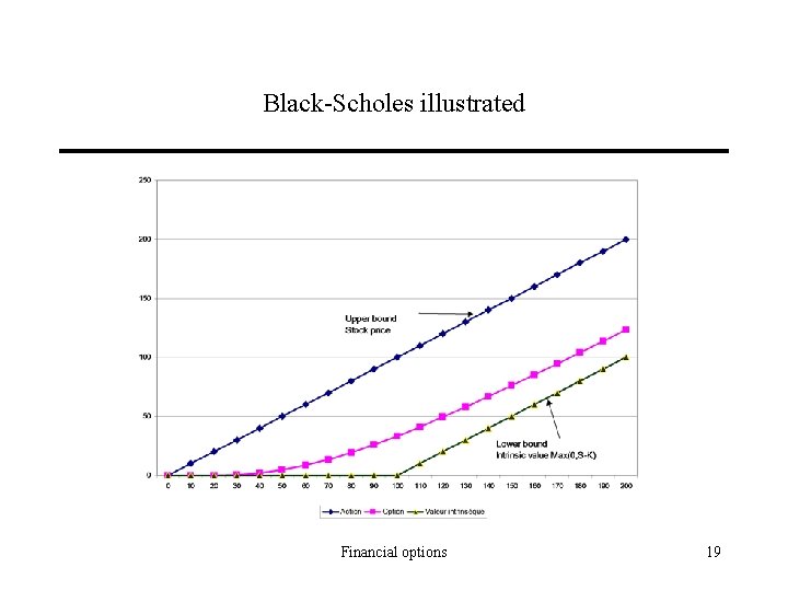
Black-Scholes illustrated Financial options 19