FROM COMPLETE LINERIZATION TO ALI AND BEYOND how

FROM COMPLETE LINERIZATION TO ALI AND BEYOND (how a somewhat younger generation built upon Dimitri’s work) Ivan Hubeny University of Arizona Collaborators: T. Lanz, D. Hummer, C. Allende-Prieto, L. Koesterke, A. Burrows, D. Sudarsky

Introduction • Stellar atmosphere (accretion disk “atmosphere”) = the region from where the photons escape to the surrounding space (and thus can be recorded by an external observer) • Radiation field is strong - it is not merely a probe of the physical state, but an important energy (momentum) balance agent • Radiation in fact determines the structure, yet its structure is probed only by radiation (exception: solar neutrinos, a few neutrinos from SN 1987 a) • Most of our knowledge about an object (a star) hinges on an understanding of its atmosphere (all basic stellar parameters) • Unlike laboratory physics, where one can change a setup of the experiment to separate various effects, we do not have this luxury in astrophysics: we are stuck with an observed spectrum • We should better make a good use of it!

Motto: One picture is worth 1000 words, but one spectrum is worth 1000 pictures!

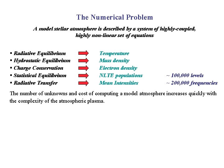
The Numerical Problem A model stellar atmosphere is described by a system of highly-coupled, highly non-linear set of equations § Radiative Equilibrium § Hydrostatic Equilibrium § Charge Conservation § Statistical Equilibrium § Radiative Transfer Temperature Mass density Electron density NLTE populations Mean Intensities ~ 100, 000 levels ~ 200, 000 frequencies The number of unknowns and cost of computing a model atmosphere increases quickly with the complexity of the atmospheric plasma.

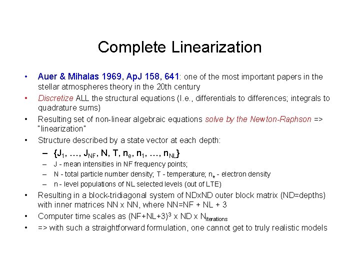
Complete Linearization • • Auer & Mihalas 1969, Ap. J 158, 641: one of the most important papers in the stellar atmospheres theory in the 20 th century Discretize ALL the structural equations (I. e. , differentials to differences; integrals to quadrature sums) Resulting set of non-linear algebraic equations solve by the Newton-Raphson => “linearization” Structure described by a state vector at each depth: – {J 1, …, JNF, N, T, ne, n 1, …, n. NL} – J - mean intensities in NF frequency points; – N - total particle number density; T - temperature; ne - electron density – n - level populations of NL selected levels (out of LTE) • • • Resulting in a block-tridiagonal system of NDx. ND outer block matrix (ND=depths) with inner matrices NN x NN, where NN=NF + NL + 3 Computer time scales as (NF+NL+3)3 x ND x Niterations => with such a straightforward formulation, one cannot get to truly realistic models

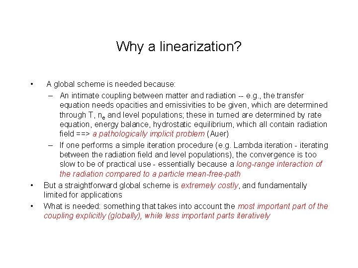
Why a linearization? • • • A global scheme is needed because: – An intimate coupling between matter and radiation -- e. g. , the transfer equation needs opacities and emissivities to be given, which are determined through T, ne and level populations; these in turned are determined by rate equation, energy balance, hydrostatic equilibrium, which all contain radiation field ==> a pathologically implicit problem (Auer) – If one performs a simple iteration procedure (e. g. Lambda iteration - iterating between the radiation field and level populations), the convergence is too slow to be of practical use - essentially because a long-range interaction of the radiation compared to a particle mean-free-path But a straightforward global scheme is extremely costly, and fundamentally limited for applications What is needed: something that takes into account the most important part of the coupling explicitly (globally), while less important parts iteratively

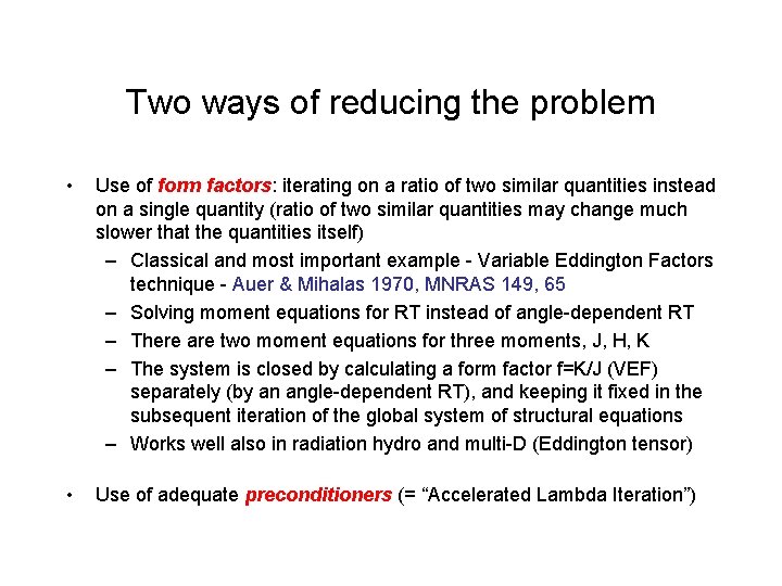
Two ways of reducing the problem • Use of form factors: iterating on a ratio of two similar quantities instead on a single quantity (ratio of two similar quantities may change much slower that the quantities itself) – Classical and most important example - Variable Eddington Factors technique - Auer & Mihalas 1970, MNRAS 149, 65 – Solving moment equations for RT instead of angle-dependent RT – There are two moment equations for three moments, J, H, K – The system is closed by calculating a form factor f=K/J (VEF) separately (by an angle-dependent RT), and keeping it fixed in the subsequent iteration of the global system of structural equations – Works well also in radiation hydro and multi-D (Eddington tensor) • Use of adequate preconditioners (= “Accelerated Lambda Iteration”)

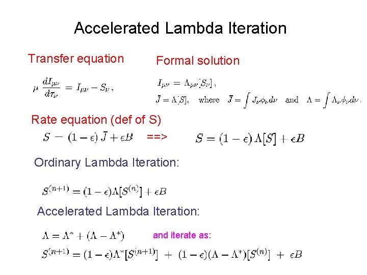
Accelerated Lambda Iteration Transfer equation Formal solution Rate equation (def of S) ==> Ordinary Lambda Iteration: Accelerated Lambda Iteration: and iterate as:

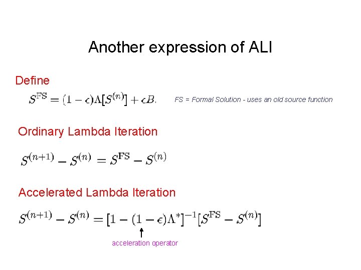
Another expression of ALI Define FS = Formal Solution - uses an old source function Ordinary Lambda Iteration Accelerated Lambda Iteration acceleration operator

Iterative solution: acceleration • • It may not be efficient to determine the next iterate solely by means of the current residuum slow convergence The rescue: to use information from previous iterates Ng acceleration - residual minimization Generally: Krylov subspace methods - using subspace spanned by (r 0, M 2 r 0, …) – Krylov subspace generally grows as we iterate • In other words: instead of using current residual, new iterate is obtained using a pseudo-residual, which is chosen to be orthogonal to the currently built Krylov subspace • • • Several (many) variants of the Krylov subspace method We selected GMRES (Generalized Minimum Residual) method, and/or Ng method A reformulated, but equivalent scheme ORTHOMIN(k) (Orthogonal minimization) – One can truncate the orthogonalization process to k most recent vectors

(future)

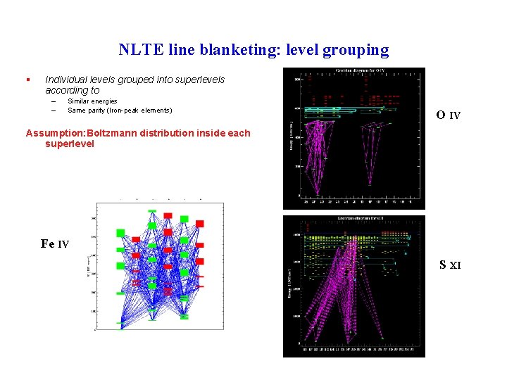
NLTE line blanketing: level grouping § Individual levels grouped into superlevels according to – – Similar energies Same parity (Iron-peak elements) O IV Assumption: Boltzmann distribution inside each superlevel Fe IV S XI

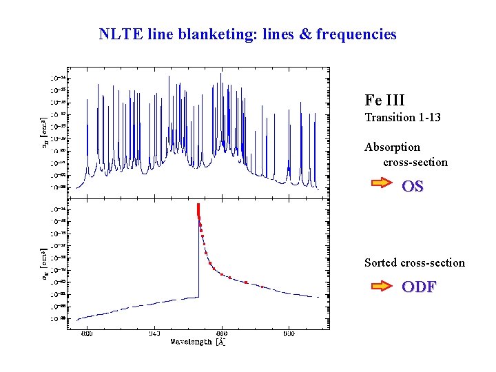
NLTE line blanketing: lines & frequencies Fe III Transition 1 -13 Absorption cross-section OS Sorted cross-section ODF

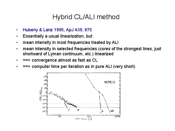
Hybrid CL/ALI method • • • Hubeny & Lanz 1995, Ap. J 439, 875 Essentially a usual linearization, but: mean intensity in most frequencies treated by ALI mean intensity in selected frequencies (cores of the strongest lines, just shortward of Lyman continuum, etc. ) linearized ==> convergence almost as fast as CL ==> computer time per iteration as in pure ALI (very short)

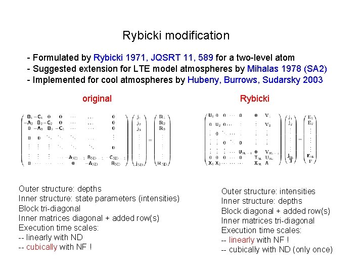
Rybicki modification - Formulated by Rybicki 1971, JQSRT 11, 589 for a two-level atom - Suggested extension for LTE model atmospheres by Mihalas 1978 (SA 2) - Implemented for cool atmospheres by Hubeny, Burrows, Sudarsky 2003 original Outer structure: depths Inner structure: state parameters (intensities) Block tri-diagonal Inner matrices diagonal + added row(s) Execution time scales: -- linearly with ND -- cubically with NF ! Rybicki Outer structure: intensities Inner structure: depths Block diagonal + added row(s) Inner matrices tri-diagonal Execution time scales: -- linearly with NF ! -- cubically with ND (only once)

TLUSTY/Cool. TLUSTY • Physics – – – – • Plane-parallel geometry Hydrostatic equilibrium Radiative + convective equilibrium Statistical equilibrium (not LTE) Computes model stellar atmospheres or accretion disks Possibility of including external irradiation (extrasolar planets) Computes model atmospheres or accretion disks Numerics – Hybrid CL/ALI method (Hubeny & Lanz 1995) – Metal line blanketing - Opacity Sampling, superleves – Rybicki solution (full CL) in Cool. Tlusty (LTE) • Range of applicability: 50 K - 109 K, with a gap 3000 -5500 K filled within the last month ------------ • Cool. TLUSTY - for brown dwarfs and extrasolar giant planets: – – Uses pre-calculated opacity and state equation tables Chemical equilibrium + departures from it Effects of clouds Circulation between the day and night side (EGP)

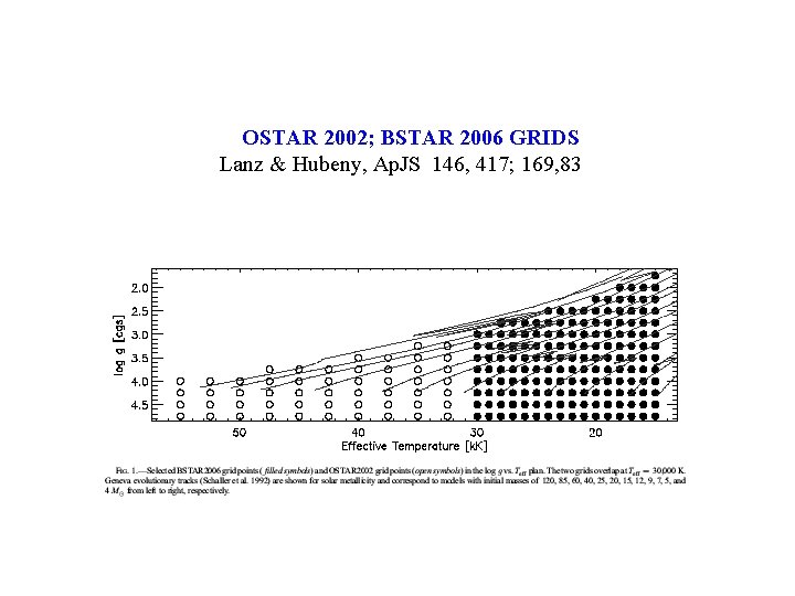
OSTAR 2002; BSTAR 2006 GRIDS Lanz & Hubeny, Ap. JS 146, 417; 169, 83

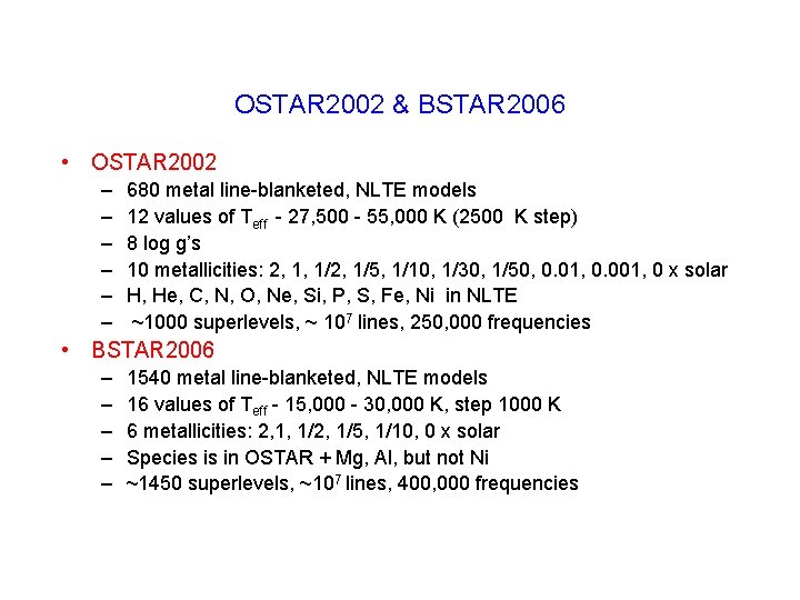
OSTAR 2002 & BSTAR 2006 • OSTAR 2002 – – – 680 metal line-blanketed, NLTE models 12 values of Teff - 27, 500 - 55, 000 K (2500 K step) 8 log g’s 10 metallicities: 2, 1, 1/2, 1/5, 1/10, 1/30, 1/50, 0. 01, 0. 001, 0 x solar H, He, C, N, O, Ne, Si, P, S, Fe, Ni in NLTE ~1000 superlevels, ~ 107 lines, 250, 000 frequencies • BSTAR 2006 – – – 1540 metal line-blanketed, NLTE models 16 values of Teff - 15, 000 - 30, 000 K, step 1000 K 6 metallicities: 2, 1, 1/2, 1/5, 1/10, 0 x solar Species is in OSTAR + Mg, Al, but not Ni ~1450 superlevels, ~107 lines, 400, 000 frequencies

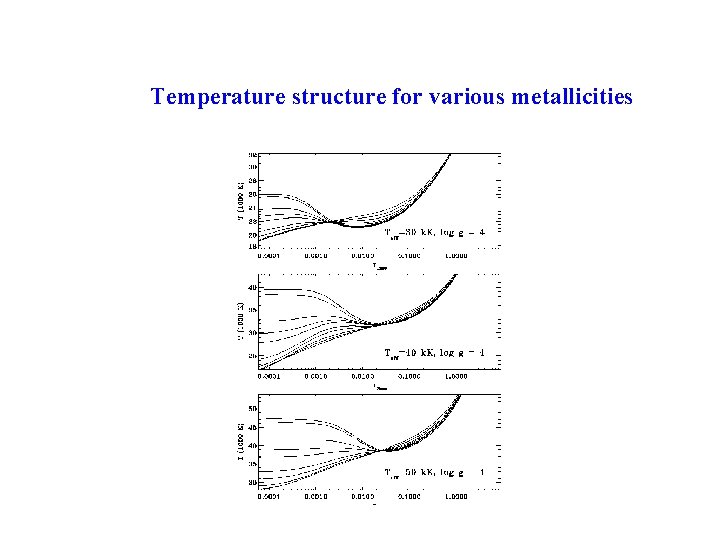
Temperature structure for various metallicities

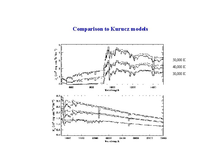
Comparison to Kurucz models 50, 000 K 40, 000 K 30, 000 K

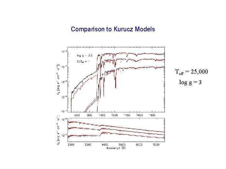
Comparison to Kurucz Models Teff = 25, 000 log g = 3

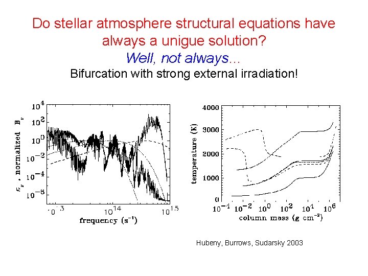
Do stellar atmosphere structural equations have always a unigue solution? Well, not always… Bifurcation with strong external irradiation! Hubeny, Burrows, Sudarsky 2003

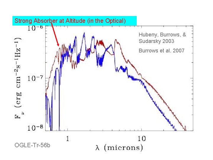
Thermal Inversion: Water in Emission (!) Strong Absorber at Altitude (in the Optical) Hubeny, Burrows, & Sudarsky 2003 Burrows et al. 2007 OGLE-Tr-56 b

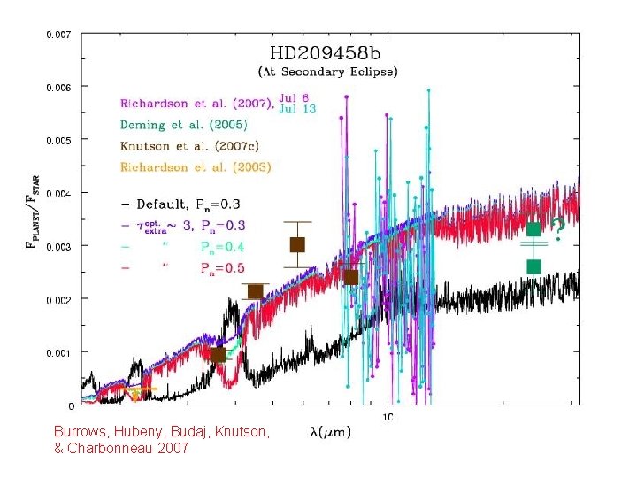
Burrows, Hubeny, Budaj, Knutson, & Charbonneau 2007

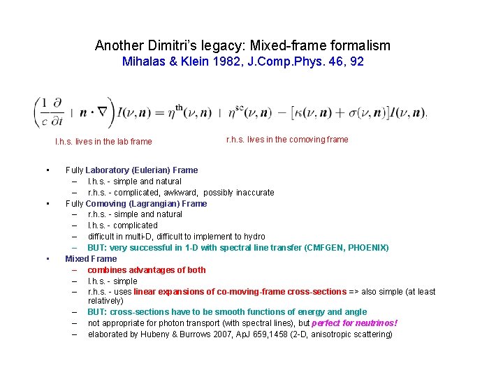
Another Dimitri’s legacy: Mixed-frame formalism Mihalas & Klein 1982, J. Comp. Phys. 46, 92 l. h. s. lives in the lab frame • • • r. h. s. lives in the comoving frame Fully Laboratory (Eulerian) Frame – l. h. s. - simple and natural – r. h. s. - complicated, awkward, possibly inaccurate Fully Comoving (Lagrangian) Frame – r. h. s. - simple and natural – l. h. s. - complicated – difficult in multi-D, difficult to implement to hydro – BUT: very successful in 1 -D with spectral line transfer (CMFGEN, PHOENIX) Mixed Frame – combines advantages of both – l. h. s. - simple – r. h. s. - uses linear expansions of co-moving-frame cross-sections => also simple (at least relatively) – BUT: cross-sections have to be smooth functions of energy and angle – not appropriate for photon transport (with spectral lines), but perfect for neutrinos! – elaborated by Hubeny & Burrows 2007, Ap. J 659, 1458 (2 -D, anisotropic scattering)

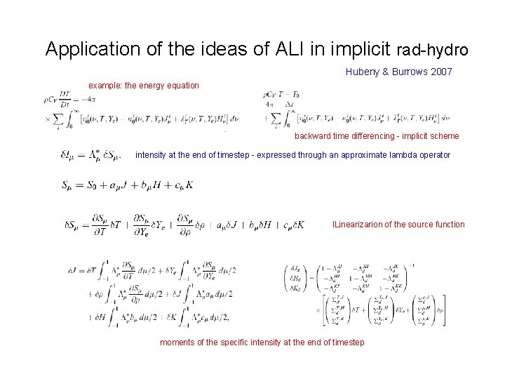
Application of the ideas of ALI in implicit rad-hydro Hubeny & Burrows 2007 example: the energy equation backward time differencing - implicit scheme intensity at the end of timestep - expressed through an approximate lambda operator l. Linearizarion of the source function moments of the specific intensity at the end of timestep

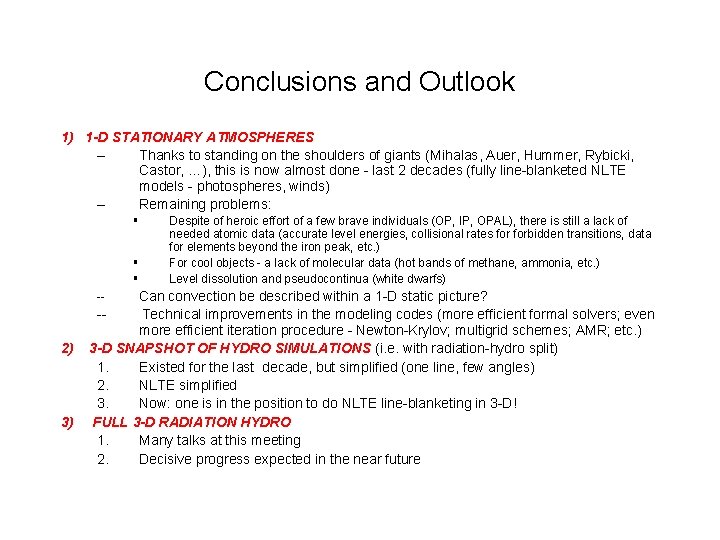
Conclusions and Outlook 1) 1 -D STATIONARY ATMOSPHERES – Thanks to standing on the shoulders of giants (Mihalas, Auer, Hummer, Rybicki, Castor, …), this is now almost done - last 2 decades (fully line-blanketed NLTE models - photospheres, winds) – Remaining problems: § § § Can convection be described within a 1 -D static picture? -Technical improvements in the modeling codes (more efficient formal solvers; even more efficient iteration procedure - Newton-Krylov; multigrid schemes; AMR; etc. ) 3 -D SNAPSHOT OF HYDRO SIMULATIONS (i. e. with radiation-hydro split) 1. Existed for the last decade, but simplified (one line, few angles) 2. NLTE simplified 3. Now: one is in the position to do NLTE line-blanketing in 3 -D! FULL 3 -D RADIATION HYDRO 1. Many talks at this meeting 2. Decisive progress expected in the near future -- 2) 3) Despite of heroic effort of a few brave individuals (OP, IP, OPAL), there is still a lack of needed atomic data (accurate level energies, collisional rates forbidden transitions, data for elements beyond the iron peak, etc. ) For cool objects - a lack of molecular data (hot bands of methane, ammonia, etc. ) Level dissolution and pseudocontinua (white dwarfs)

Dimitri, we all salute you!