Frequent Item Mining What is data mining Pattern

Frequent Item Mining

What is data mining? • =Pattern Mining? • What patterns? • Why are they useful?

Definition: Frequent Itemset • Itemset – A collection of one or more items • Example: {Milk, Bread, Diaper} – k-itemset • An itemset that contains k items • Support count ( ) – Frequency of occurrence of an itemset – E. g. ({Milk, Bread, Diaper}) = 2 • Support – Fraction of transactions that contain an itemset – E. g. s({Milk, Bread, Diaper}) = 2/5 • Frequent Itemset – An itemset whose support is greater than or equal to a minsup threshold 3

Frequent Itemsets Mining TID Transactions 100 { A, B, E } 200 { B, D } 300 { A, B, E } 400 { A, C } 500 { B, C } 600 { A, C } 700 { A, B } 800 { A, B, C, E } 900 { A, B, C } 1000 { A, C, E } • Minimum support level 50% – {A}, {B}, {C}, {A, B}, {A, C}

Three Different Views of FIM • Transactional Database – How we do store a transactional database? • Horizontal, Vertical, Transaction-Item Pair • Binary Matrix • Bipartite Graph • How does the FIM formulated in these different settings? 5

Frequent Itemset Generation Given d items, there are 2 d possible candidate itemsets 6

Frequent Itemset Generation • Brute-force approach: – Each itemset in the lattice is a candidate frequent itemset – Count the support of each candidate by scanning the database – Match each transaction against every candidate – Complexity ~ O(NMw) => Expensive since M = 2 d !!! 7

Reducing Number of Candidates • Apriori principle: – If an itemset is frequent, then all of its subsets must also be frequent • Apriori principle holds due to the following property of the support measure: – Support of an itemset never exceeds the support of its subsets – This is known as the anti-monotone property of support 8

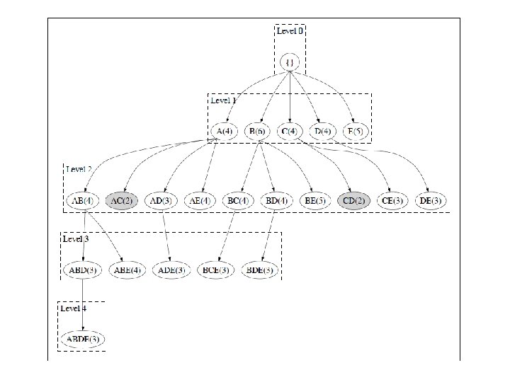
Illustrating Apriori Principle Found to be Infrequent Pruned supersets 9

Illustrating Apriori Principle Items (1 -itemsets) Pairs (2 -itemsets) (No need to generate candidates involving Coke or Eggs) Minimum Support = 3 Triplets (3 -itemsets) If every subset is considered, 6 C + 6 C = 41 1 2 3 With support-based pruning, 6 + 1 = 13 10

Apriori R. Agrawal and R. Srikant. Fast algorithms for mining association rules. VLDB, 487 -499, 1994

How to Generate Candidates? • Suppose the items in Lk-1 are listed in an order • Step 1: self-joining Lk-1 insert into Ck select p. item 1, p. item 2, …, p. itemk-1, q. itemk-1 from Lk-1 p, Lk-1 q where p. item 1=q. item 1, …, p. itemk-2=q. itemk-2, p. itemk-1 < q. itemk-1 • Step 2: pruning forall itemsets c in Ck do forall (k-1)-subsets s of c do if (s is not in Lk-1) then delete c from Ck 13

Challenges of Frequent Itemset Mining • Challenges – Multiple scans of transaction database – Huge number of candidates – Tedious workload of support counting for candidates • Improving Apriori: general ideas – Reduce passes of transaction database scans – Shrink number of candidates – Facilitate support counting of candidates 14

Alternative Methods for Frequent Itemset Generation • Representation of Database – horizontal vs vertical data layout 15

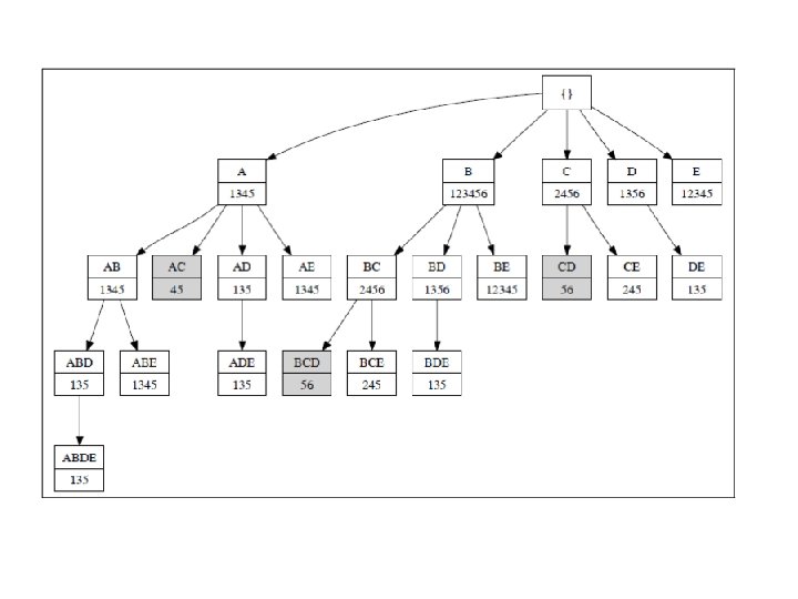
ECLAT • For each item, store a list of transaction ids (tids) TID-list 16

ECLAT • Determine support of any k-itemset by intersecting tid-lists of two of its (k-1) subsets. • 3 traversal approaches: – top-down, bottom-up and hybrid • Advantage: very fast support counting • Disadvantage: intermediate tid-lists may become too large for memory 17

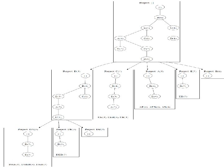
FP-growth Algorithm • Use a compressed representation of the database using an FP-tree • Once an FP-tree has been constructed, it uses a recursive divide-and-conquer approach to mine the frequent itemsets 20

FP-tree construction null After reading TID=1: A: 1 B: 1 After reading TID=2: A: 1 B: 1 null B: 1 C: 1 D: 1 21

FP-Tree Construction Transaction Database null B: 3 A: 7 B: 5 Header table C: 1 C: 3 D: 1 D: 1 E: 1 Pointers are used to assist frequent itemset generation 22

FP-growth C: 1 Conditional Pattern base for D: P = {(A: 1, B: 1, C: 1), (A: 1, B: 1), (A: 1, C: 1), (A: 1), (B: 1, C: 1)} D: 1 Recursively apply FPgrowth on P null A: 7 B: 5 C: 1 C: 3 D: 1 B: 1 D: 1 Frequent Itemsets found (with sup > 1): AD, BD, CD, ACD, BCD 23

Compact Representation of Frequent Itemsets • Some itemsets are redundant because they have identical support as their supersets • Number of frequent itemsets • Need a compact representation 25

Maximal Frequent Itemset An itemset is maximal frequent if none of its immediate supersets is frequent Maximal Itemsets Infrequent Itemsets Border 26

Closed Itemset • An itemset is closed if none of its immediate supersets has the same support as the itemset 27

Maximal vs Closed Itemsets Transaction Ids Not supported by any transactions 28

Maximal vs Closed Frequent Itemsets Minimum support = 2 Closed but not maximal Closed and maximal # Closed = 9 # Maximal = 4 29

Maximal vs Closed Itemsets 30

Association Rule Mining and FIM

Research Questions • How to efficiently enumerate Maximal Frequent Itemsets? • How about Closed Frequent Itemsets? 32

Association Rule Mining • Given a set of transactions, find rules that will predict the occurrence of an item based on the occurrences of other items in the transaction Example of Association Rules Market-Basket transactions {Diaper} {Beer}, {Beer, Bread} {Milk}, Implication means co-occurrence, not causality! 33

Definition: Association Rule p Association Rule n n p An implication expression of the form X Y, where X and Y are itemsets Example: {Milk, Diaper} {Beer} Rule Evaluation Metrics n Support (s) p n Fraction of transactions that contain both X and Y Example: Confidence (c) p Measures how often items in Y appear in transactions that contain X 34

Association Rule Mining Task • Given a set of transactions T, the goal of association rule mining is to find all rules having – support ≥ minsup threshold – confidence ≥ minconf threshold • Brute-force approach: – List all possible association rules – Compute the support and confidence for each rule – Prune rules that fail the minsup and minconf thresholds Computationally prohibitive! 35

Mining Association Rules Example of Rules: {Milk, Diaper} {Beer} (s=0. 4, c=0. 67) {Milk, Beer} {Diaper} (s=0. 4, c=1. 0) {Diaper, Beer} {Milk} (s=0. 4, c=0. 67) {Beer} {Milk, Diaper} (s=0. 4, c=0. 67) {Diaper} {Milk, Beer} (s=0. 4, c=0. 5) {Milk} {Diaper, Beer} (s=0. 4, c=0. 5) Observations: • All the above rules are binary partitions of the same itemset: {Milk, Diaper, Beer} • Rules originating from the same itemset have identical support but can have different confidence • Thus, we may decouple the support and confidence requirements 36

Mining Association Rules • Two-step approach: 1. Frequent Itemset Generation – Generate all itemsets whose support minsup 2. Rule Generation – Generate high confidence rules from each frequent itemset, where each rule is a binary partitioning of a frequent itemset • Frequent itemset generation is still computationally expensive 37

Computational Complexity • Given d unique items: – Total number of itemsets = 2 d – Total number of possible association rules: If d=6, R = 602 rules 38

Rule Generation • Given a frequent itemset L, find all non-empty subsets f L such that f L – f satisfies the minimum confidence requirement – If {A, B, C, D} is a frequent itemset, candidate rules: ABC D, A BCD, AB CD, BD AC, ABD C, B ACD, AC BD, CD AB, ACD B, C ABD, AD BC, BCD A, D ABC BC AD, • If |L| = k, then there are 2 k – 2 candidate association rules (ignoring L and L) 39

Rule Generation • How to efficiently generate rules from frequent itemsets? – In general, confidence does not have an antimonotone property c(ABC D) can be larger or smaller than c(AB D) – But confidence of rules generated from the same itemset has an anti-monotone property – e. g. , L = {A, B, C, D}: c(ABC D) c(AB CD) c(A BCD) • Confidence is anti-monotone w. r. t. number of items on the RHS of the rule 40

Rule Generation for Apriori Algorithm Lattice of rules Low Confidence Rule Pruned Rules 41

Rule Generation for Apriori Algorithm • Candidate rule is generated by merging two rules that share the same prefix in the rule consequent • join(CD=>AB, BD=>AC) would produce the candidate rule D => ABC • Prune rule D=>ABC if its subset AD=>BC does not have high confidence 42

Beyond Itemsets • Sequence Mining – Finding frequent subsequences from a collection of sequences • Graph Mining – Finding frequent (connected) subgraphs from a collection of graphs • Tree Mining – Finding frequent (embedded) subtrees from a set of trees/graphs • Geometric Structure Mining – Finding frequent substructures from 3 -D or 2 -D geometric graphs • Among others…

Frequent Pattern Mining E A A E B A B D A C F D D E B E A A B F B A C F A B D C D F D C C

Why Frequent Pattern Mining is So Important? • Application Domains – Business, biology, chemistry, WWW, computer/networing security, … • Summarizing the underlying datasets, providing key insights • Basic tools for other data mining tasks – – – Assocation rule mining Classification Clustering Change Detection etc…

Network motifs: recurring patterns that occur significantly more than in randomized nets • Do motifs have specific roles in the network? • Many possible distinct subgraphs

The 13 three-node connected subgraphs

199 4 -node directed connected subgraphs And it grows fast for larger subgraphs : 9364 5 -node subgraphs, 1, 530, 843 6 -node…

Finding network motifs – an overview • Generation of a suitable random ensemble (reference networks) • Network motifs detection process: p p Count how many times each subgraph appears Compute statistical significance for each subgraph – probability of appearing in random as much as in real network (P-val or Z-score)

Ensemble of networks Real = 5 Rand=0. 5± 0. 6 Zscore (#Standard Deviations)=7. 5

Performance and Scalability: Apriori Implementation

Apriori R. Agrawal and R. Srikant. Fast algorithms for mining association rules. VLDB, 487 -499, 1994

Challenges of Frequent Itemset Mining • Challenges – Multiple scans of transaction database – Huge number of candidates – Tedious workload of support counting for candidates • Improving Apriori: general ideas – Reduce passes of transaction database scans – Shrink number of candidates – Facilitate support counting of candidates 53

Reducing Number of Comparisons • Candidate counting: – Scan the database of transactions to determine the support of each candidate itemset – To reduce the number of comparisons, store the candidates in a hash structure • Instead of matching each transaction against every candidate, match it against candidates contained in the hashed buckets

Generate Hash Tree Suppose you have 15 candidate itemsets of length 3: {1 4 5}, {1 2 4}, {4 5 7}, {1 2 5}, {4 5 8}, {1 5 9}, {1 3 6}, {2 3 4}, {5 6 7}, {3 4 5}, {3 5 6}, {3 5 7}, {6 8 9}, {3 6 7}, {3 6 8} You need: • Hash function • Max leaf size: max number of itemsets stored in a leaf node (if number of candidate itemsets exceeds max leaf size, split the node) Hash function 3, 6, 9 1, 4, 7 234 567 345 136 145 2, 5, 8 124 457 125 458 159 356 357 689 367 368

Association Rule Discovery: Hash tree Hash Function 1, 4, 7 Candidate Hash Tree 3, 6, 9 2, 5, 8 234 567 145 Hash on 1, 4 or 7 136 345 124 125 457 458 159 356 357 689 367 368

Association Rule Discovery: Hash tree Hash Function 1, 4, 7 Candidate Hash Tree 3, 6, 9 2, 5, 8 234 567 145 Hash on 2, 5 or 8 136 345 124 125 457 458 159 356 357 689 367 368

Association Rule Discovery: Hash tree Hash Function 1, 4, 7 Candidate Hash Tree 3, 6, 9 2, 5, 8 234 567 145 Hash on 3, 6 or 9 136 345 124 125 457 458 159 356 357 689 367 368

Subset Operation Given a transaction t, what are the possible subsets of size 3?

Subset Operation Using Hash Tree Hash Function 1 2 3 5 6 transaction 1+ 2356 2+ 356 1, 4, 7 3+ 56 234 567 145 136 345 124 457 125 458 159 356 357 689 367 368 2, 5, 8 3, 6, 9

Subset Operation Using Hash Tree Hash Function 1 2 3 5 6 transaction 1+ 2356 2+ 356 1, 4, 7 3+ 56 13+ 56 234 567 15+ 6 145 136 345 124 457 125 458 159 356 357 689 367 368 2, 5, 8 3, 6, 9

Subset Operation Using Hash Tree Hash Function 1 2 3 5 6 transaction 1+ 2356 2+ 356 1, 4, 7 3+ 56 3, 6, 9 2, 5, 8 13+ 56 234 567 15+ 6 145 136 345 124 457 125 458 159 356 357 689 367 368 Match transaction against 11 out of 15 candidates

Prefix Tree Representation Efficient Implementations of Apriori and Eclat Christian Borgelt. , FIMI’ 03

Prefix Tree

Prefix Tree Structure for Counting

Other key optimization • Recording the items – Why is this relevant? • Transaction Tree – Organize transaction into trees – Count through two trees

Scalability • How to handle very large dataset? • The dataset can not be stored in the main memory • Performance of out-of-core datasets/Performance of in-core datasets

Partition: Scan Database Only Twice • Any itemset that is potentially frequent in DB must be frequent in at least one of the partitions of DB – Scan 1: partition database and find local frequent patterns – Scan 2: consolidate global frequent patterns • A. Savasere, E. Omiecinski, and S. Navathe. An efficient algorithm for mining association in large databases. In VLDB’ 95

DHP: Reduce the Number of Candidates • A k-itemset whose corresponding hashing bucket count is below the threshold cannot be frequent – Candidates: a, b, c, d, e – Hash entries: {ab, ad, ae} {bd, be, de} … – Frequent 1 -itemset: a, b, d, e – ab is not a candidate 2 -itemset if the sum of count of {ab, ad, ae} is below support threshold • J. Park, M. Chen, and P. Yu. An effective hash-based algorithm for mining association rules. In SIGMOD’ 95

Sampling for Frequent Patterns • Select a sample of original database, mine frequent patterns within sample using Apriori • Scan database once to verify frequent itemsets found in sample, only borders of closure of frequent patterns are checked – Example: check abcd instead of ab, ac, …, etc. • Scan database again to find missed frequent patterns • H. Toivonen. Sampling large databases for association rules. In VLDB’ 96

DIC: Reduce Number of Scans ABCD • ABC ABD ACD BCD AB AC BC AD BD • CD Once both A and D are determined frequent, the counting of AD begins Once all length-2 subsets of BCD are determined frequent, the counting of BCD begins Transactions B A C D Apriori {} Itemset lattice S. Brin R. Motwani, J. Ullman, and S. Tsur. Dynamic itemset DIC counting and implication rules for market basket data. In SIGMOD’ 97 1 -itemsets 2 -itemsets … 1 -itemsets 2 -items 3 -items

References • R. Agrawal, T. Imielinski, and A. Swami. Mining association rules between sets of items in large databases. SIGMOD, 207 -216, 1993. • R. Agrawal and R. Srikant. Fast algorithms for mining association rules. VLDB, 487 -499, 1994. • R. J. Bayardo. Efficiently mining long patterns from databases. SIGMOD, 85 -93, 1998. 72

References: • Christian Borgelt, Efficient Implementations of Apriori and Eclat, FIMI’ 03 • Ferenc Bodon, A fast APRIORI implementation, FIMI’ 03 • Ferenc Bodon, A Survey on Frequent Itemset Mining, Technical Report, Budapest University of Technology and Economic, 2006

Important websites: • FIMI workshop – Not only Apriori and FIM • FP-tree, ECLAT, Closed, Maximal – http: //fimi. cs. helsinki. fi/ • Christian Borgelt’s website – http: //www. borgelt. net/software. html • Ferenc Bodon’s website – http: //www. cs. bme. hu/~bodon/en/apriori/