Frequency and Severity vs Loss Cost Modeling CAS

Frequency and Severity vs. Loss Cost Modeling CAS 2012 Ratemaking and Product Management Seminar March 2012 Philadelphia, PA Alietia Caughron, Ph. D Homesite Insurance Group Privileged & Confidential

Antitrust Notice • The Casualty Actuarial Society is committed to adhering strictly to the letter and spirit of the antitrust laws. Seminars conducted under the auspices of the CAS are designed solely to provide a forum for the expression of various points of view on topics described in the programs or agendas for such meetings. • Under no circumstances shall CAS seminars be used as a means for competing companies or firms to reach any understanding – expressed or implied – that restricts competition or in any way impairs the ability of members to exercise independent business judgment regarding matters affecting competition. • It is the responsibility of all seminar participants to be aware of antitrust regulations, to prevent any written or verbal discussions that appear to violate these laws, and to adhere in every respect to the CAS antitrust compliance policy. Privileged & Confidential 2

Agenda q Motivation q Example Privileged & Confidential 3

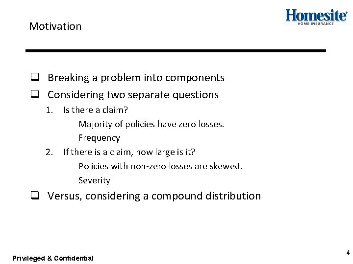
Motivation q Breaking a problem into components q Considering two separate questions 1. Is there a claim? Majority of policies have zero losses. Frequency 2. If there is a claim, how large is it? Policies with non-zero losses are skewed. Severity q Versus, considering a compound distribution Privileged & Confidential 4

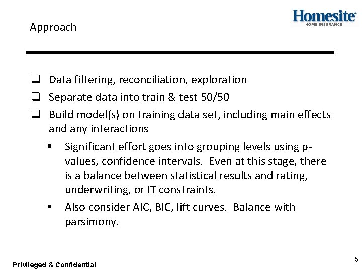
Approach q Data filtering, reconciliation, exploration q Separate data into train & test 50/50 q Build model(s) on training data set, including main effects and any interactions § Significant effort goes into grouping levels using pvalues, confidence intervals. Even at this stage, there is a balance between statistical results and rating, underwriting, or IT constraints. § Also consider AIC, BIC, lift curves. Balance with parsimony. Privileged & Confidential 5

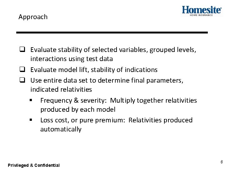
Approach q Evaluate stability of selected variables, grouped levels, interactions using test data q Evaluate model lift, stability of indications q Use entire data set to determine final parameters, indicated relativities § Frequency & severity: Multiply together relativities produced by each model § Loss cost, or pure premium: Relativities produced automatically Privileged & Confidential 6

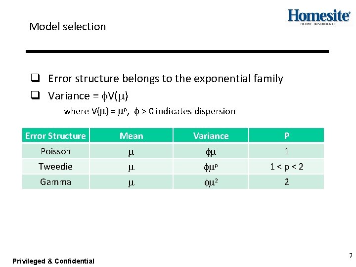
Model selection q Error structure belongs to the exponential family q Variance = f. V(m) where V(m) = mp, f > 0 indicates dispersion Error Structure Mean Variance P Poisson m fm 1 Tweedie m fmp 1<p<2 Gamma m fm 2 2 Privileged & Confidential 7

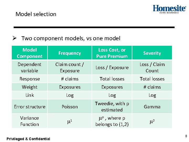
Model selection Ø Two component models, vs one model Model Component Frequency Loss Cost, or Pure Premium Severity Dependent variable Claim count / Exposure Loss / Claim Count Response # claims Total losses Weight Exposures # claims Link Log Log Error structure Poisson Tweedie, with p estimated Gamma Variance Function m 1 mp , where p belongs to (1, 2) m 2 Privileged & Confidential 8

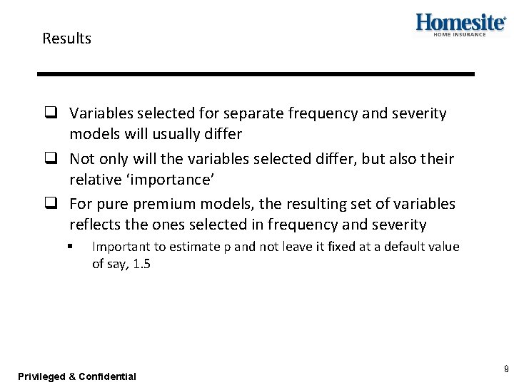
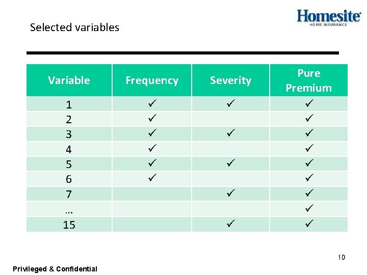
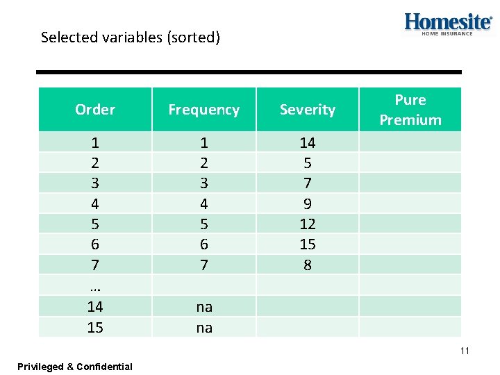
Results q Variables selected for separate frequency and severity models will usually differ q Not only will the variables selected differ, but also their relative ‘importance’ q For pure premium models, the resulting set of variables reflects the ones selected in frequency and severity § Important to estimate p and not leave it fixed at a default value of say, 1. 5 Privileged & Confidential 9

Selected variables Variable Frequency Severity 1 2 3 4 5 6 7 … 15 ü ü ü Pure Premium ü ü ü ü ü 10 Privileged & Confidential

Selected variables (sorted) Order Frequency Severity 1 2 3 4 5 6 7 … 14 15 1 2 3 4 5 6 7 14 5 7 9 12 15 8 Pure Premium na na 11 Privileged & Confidential

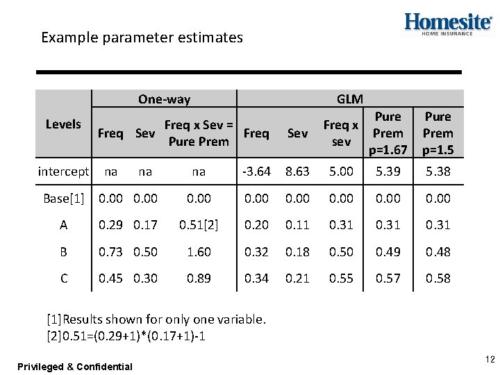
Example parameter estimates One-way Levels intercept GLM Freq x Sev = Freq Sev Freq Pure Prem na na Base[1] 0. 00 Sev Freq x sev Pure Prem p=1. 67 Pure Prem p=1. 5 na -3. 64 8. 63 5. 00 5. 39 5. 38 0. 00 A 0. 29 0. 17 0. 51[2] 0. 20 0. 11 0. 31 B 0. 73 0. 50 1. 60 0. 32 0. 18 0. 50 0. 49 0. 48 C 0. 45 0. 30 0. 89 0. 34 0. 21 0. 55 0. 57 0. 58 [1]Results shown for only one variable. [2]0. 51=(0. 29+1)*(0. 17+1)-1 Privileged & Confidential 12

Example relativities One-way[1] Levels intercept GLM Freq x Sev = Freq Sev Freq Pure Prem na na Base[1] 1. 00 na Sev 2. 64% 5, 614 Freq x sev Pure Prem p=1. 67 Pure Prem p=1. 5 148 219 218 1. 00 A 1. 34 1. 18 1. 66 [2] 1. 22 1. 11 1. 36 B 2. 08 1. 65 4. 94 1. 37 1. 20 1. 64 1. 63 1. 61 C 1. 57 1. 36 2. 44 1. 41 1. 23 1. 74 1. 77 1. 78 [1]Results shown for only one variable. [2]1. 66=exp(0. 51) Privileged & Confidential 13

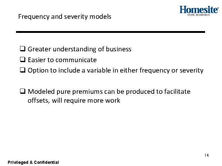
Frequency and severity models q Greater understanding of business q Easier to communicate q Option to include a variable in either frequency or severity q Modeled pure premiums can be produced to facilitate offsets, will require more work 14 Privileged & Confidential

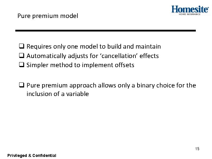
Pure premium model q Requires only one model to build and maintain q Automatically adjusts for ‘cancellation’ effects q Simpler method to implement offsets q Pure premium approach allows only a binary choice for the inclusion of a variable 15 Privileged & Confidential

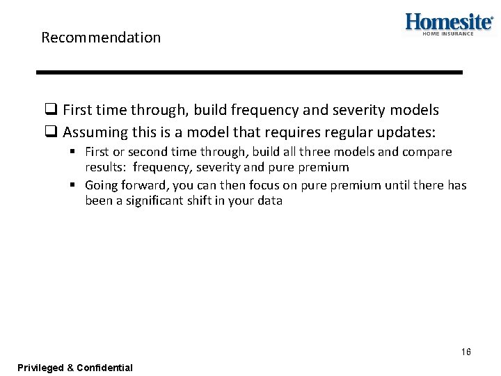
Recommendation q First time through, build frequency and severity models q Assuming this is a model that requires regular updates: § First or second time through, build all three models and compare results: frequency, severity and pure premium § Going forward, you can then focus on pure premium until there has been a significant shift in your data 16 Privileged & Confidential

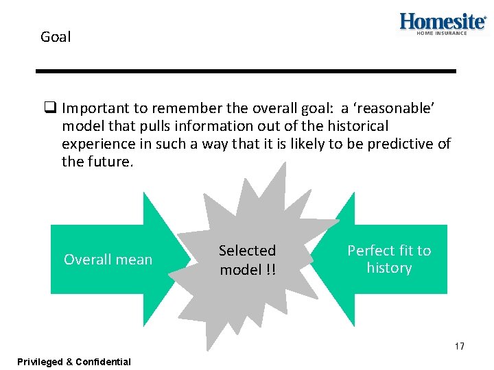
Goal q Important to remember the overall goal: a ‘reasonable’ model that pulls information out of the historical experience in such a way that it is likely to be predictive of the future. Overall mean Selected model !! Perfect fit to history 17 Privileged & Confidential