Frederick Kingdom Frederick Kingdom Photo Georges Jansoon Illusion

Frederick Kingdom

Frederick Kingdom

Photo: Georges Jansoon. Illusion: Frederick Kingdom, Ali Yoonessi and Elena

Frederick Kingdom

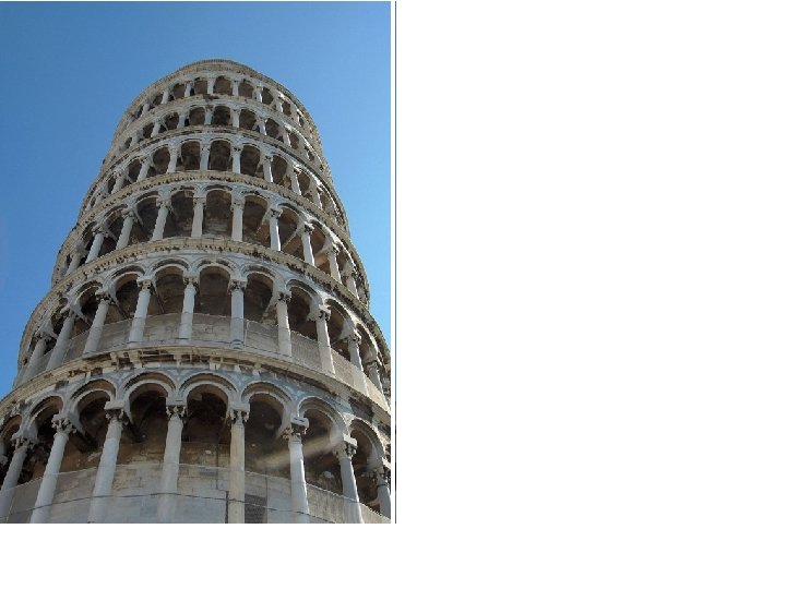
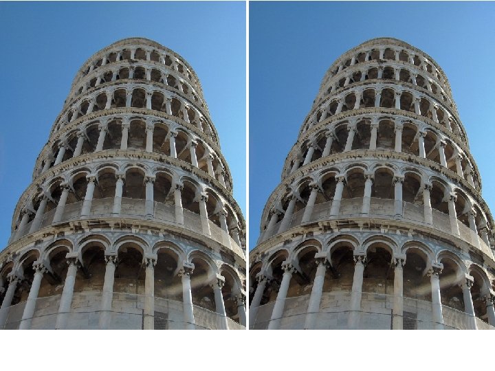
Depth from disparity • Goal: recover depth by finding image coordinate x’ that corresponds to x X X z x x x' x’ f O f Baseline T O’

Geometry for a simple stereo system • Assume parallel optical axes, known camera parameters (i. e. , calibrated cameras). What is expression for Z? Similar triangles (pl, P, pr) and (Ol, P, Or): disparity

Depth from disparity • Goal: recover depth by finding image coordinate x’ that corresponds to x • Sub-Problems 1. Calibration: How do we recover the relation of the cameras (if not already known)? 2. Correspondence: How do we search for the matching point x’? X x x'

Depth from disparity image I(x, y) Disparity map D(x, y) image I´(x´, y´)=(x+D(x, y) If we could find the corresponding points in two images, we could estimate relative depth… James Hays

What do we need to know? 1. Calibration for the two cameras. 1. Intrinsic matrices for both cameras (e. g. , f) 2. Baseline distance T in parallel camera case 3. R, t in non-parallel case 2. Correspondence for every pixel. Like project 2, but project 2 is “sparse”. We need “dense” correspondence!

Correspondence for every pixel. Where do we need to search?

Wouldn’t it be nice to know where matches can live? Epipolar geometry Constrains 2 D search to 1 D

Key idea: Epipolar constraint X X X x x’ x’ x’ Potential matches for x’ have to lie on the corresponding line l. Potential matches for x have to lie on the corresponding line l’.

Epipolar geometry: notation X x x’ • Baseline – line connecting the two camera centers • Epipoles = intersections of baseline with image planes = projections of the other camera center • Epipolar Plane – plane containing baseline (1 D family)

Epipolar geometry: notation X x x’ • Baseline – line connecting the two camera centers • Epipoles = intersections of baseline with image planes = projections of the other camera center • Epipolar Plane – plane containing baseline (1 D family) • Epipolar Lines - intersections of epipolar plane with image planes (always come in corresponding pairs)

= camera center Think Pair Share Where are the epipoles? What do the epipolar lines look like? a) c) X X b) d) X X

Example: Converging cameras

Example: Motion parallel to image plane

Example: Forward motion e’ e Epipole has same coordinates in both images. Points move along lines radiating from e: “Focus of expansion”

What is this useful for? X x x’ • Find X: If I know x, and have calibrated cameras (known intrinsics K, K’ and extrinsic relationship), I can restrict x’ to be along l’. • Discover disparity for stereo.

What is this useful for? X x x’ • Given candidate x, x’ correspondences, estimate relative position and orientation between the cameras and the 3 D position of corresponding image points.

What is this useful for? X x x’ • Model fitting: see if candidate x, x’ correspondences fit estimated projection models of cameras 1 and 2.

Epipolar lines

Keep only the matches at are “inliers” with respect to the “best” fundamental matrix

Epipolar constraint: Calibrated case X Homogeneous 2 d point (3 D ray towards X) x x’ 3 D scene point 2 D pixel coordinate (homogeneous) 3 D scene point in 2 nd camera’s 3 D coordinates

Epipolar constraint: Calibrated case X Homogeneous 2 d point (3 D ray towards X) x x’ 3 D scene point 2 D pixel coordinate (homogeneous) 3 D scene point in 2 nd camera’s 3 D coordinates

Essential matrix X x x’ E is a 3 x 3 matrix which relates corresponding pairs of normalized homogeneous image points across pairs of images – for K calibrated cameras. Estimates relative position/orientation. Essential Matrix (Longuet-Higgins, 1981) Note: [t]× is matrix representation of cross product

Epipolar constraint: Uncalibrated case X x x’ • If we don’t know K and K’, then we can write the epipolar constraint in terms of unknown normalized coordinates:

The Fundamental Matrix Without knowing K and K’, we can define a similar relation using unknown normalized coordinates Fundamental Matrix (Faugeras and Luong, 1992)

Properties of the Fundamental matrix X x x’ • • F x’ = 0 is the epipolar line l associated with x’ FTx = 0 is the epipolar line l’ associated with x • • • F is singular (rank two): det(F)=0 F e’ = 0 and FTe = 0 (nullspaces of F = e’; nullspace of FT = e’) F has seven degrees of freedom: 9 entries but defined up to scale, det(F)=0

F in more detail •

Estimating the Fundamental Matrix • 8 -point algorithm – Least squares solution using SVD on equations from 8 pairs of correspondences – Enforce det(F)=0 constraint using SVD on F Note: estimation of F (or E) is degenerate for a planar scene.

8 -point algorithm 1. Solve a system of homogeneous linear equations a. Write down the system of equations

8 -point algorithm 1. Solve a system of homogeneous linear equations a. Write down the system of equations b. Solve f from Af=0 using SVD Matlab: [U, S, V] = svd(A); f = V(: , end); F = reshape(f, [3 3])’;

Need to enforce singularity constraint

8 -point algorithm 1. Solve a system of homogeneous linear equations a. Write down the system of equations b. Solve f from Af=0 using SVD Matlab: [U, S, V] = svd(A); f = V(: , end); F = reshape(f, [3 3])’; 2. Resolve det(F) = 0 constraint using SVD Matlab: [U, S, V] = svd(F); S(3, 3) = 0; F = U*S*V’;

Problem with eight-point algorithm

Problem with eight-point algorithm Poor numerical conditioning Can be fixed by rescaling the data

The normalized eight-point algorithm (Hartley, 1995) • Center the image data at the origin, and scale it so the mean squared distance between the origin and the data points is 2 pixels • Use the eight-point algorithm to compute F from the normalized points • Enforce the rank-2 constraint (for example, take SVD of F and throw out the smallest singular value) • Transform fundamental matrix back to original units: if T and T’ are the normalizing transformations in the two images, than the fundamental matrix in original coordinates is T’T F T

Comparison of estimation algorithms 8 -point Normalized 8 -point Nonlinear least squares Av. Dist. 1 2. 33 pixels 0. 92 pixel 0. 86 pixel Av. Dist. 2 2. 18 pixels 0. 85 pixel 0. 80 pixel

From epipolar geometry to camera calibration • If we know the calibration matrices of the two cameras, we can estimate the essential matrix: E = KTFK’ • The essential matrix gives us the relative rotation and translation between the cameras, or their extrinsic parameters. • Fundamental matrix lets us compute relationship up to scale for cameras with unknown intrinsic calibrations. • Estimating the fundamental matrix is a kind of “weak calibration”

Let’s recap… • Fundamental matrix song • http: //danielwedge. com/fmatrix/

Among all my matches, how do I know which ones are good?

VLFeat’s 800 most confident matches among 10, 000+ local features.

Least squares: Robustness to noise • Least squares fit to the red points:

Least squares: Robustness to noise • Least squares fit with an outlier: Problem: squared error heavily penalizes outliers

Least squares line fitting • Data: (x 1, y 1), …, (xn, yn) • Line equation: yi = m xi + b • Find (m, b) to minimize y=mx+b (xi, yi) Matlab: p = A y; (Closed form solution) Modified from S. Lazebnik

Robust least squares (to deal with outliers) General approach: minimize ui (xi, θ) – residual of ith point w. r. t. model parameters ϴ ρ – robust function with scale parameter σ The robust function ρ • Favors a configuration with small residuals • Constant penalty for large residuals Slide from S. Savarese

Choosing the scale: Just right The effect of the outlier is minimized

Choosing the scale: Too small The error value is almost the same for every point and the fit is very poor

Choosing the scale: Too large Behaves much the same as least squares

Robust estimation: Details • Robust fitting is a nonlinear optimization problem that must be solved iteratively • Scale of robust function should be chosen adaptively based on median residual • Least squares solution can be used for initialization

VLFeat’s 800 most confident matches among 10, 000+ local features.

RANSAC (RANdom SAmple Consensus) : Fischler & Bolles in ‘ 81.

RANSAC (RANdom SAmple Consensus) : Fischler & Bolles in ‘ 81.

RANSAC (RANdom SAmple Consensus) : Fischler & Bolles in ‘ 81. This data is noisy, but we expect a good fit to a known model.

RANSAC (RANdom SAmple Consensus) : Fischler & Bolles in ‘ 81. This data is noisy, but we expect a good fit to a known model. Here, we expect to see a line, but leastsquares fitting will produce the wrong result due to strong outlier presence.

RANSAC (RANdom SAmple Consensus) : Fischler & Bolles in ‘ 81. Algorithm: 1. Sample (randomly) the number of points s required to fit the model 2. Solve for model parameters using samples 3. Score by the fraction of inliers within a preset threshold of the model Repeat 1 -3 until the best model is found with high confidence

RANSAC Line fitting example Algorithm: 1. Sample (randomly) the number of points required to fit the model (s=2) 2. Solve for model parameters using samples 3. Score by the fraction of inliers within a preset threshold of the model Repeat 1 -3 until the best model is found with high confidence Illustration by Savarese

RANSAC Line fitting example Algorithm: 1. Sample (randomly) the number of points required to fit the model (s=2) 2. Solve for model parameters using samples 3. Score by the fraction of inliers within a preset threshold of the model Repeat 1 -3 until the best model is found with high confidence

RANSAC Line fitting example Algorithm: 1. Sample (randomly) the number of points required to fit the model (s=2) 2. Solve for model parameters using samples 3. Score by the fraction of inliers within a preset threshold of the model Repeat 1 -3 until the best model is found with high confidence

RANSAC Algorithm: 1. Sample (randomly) the number of points required to fit the model (s=2) 2. Solve for model parameters using samples 3. Score by the fraction of inliers within a preset threshold of the model Repeat 1 -3 until the best model is found with high confidence

How to choose parameters? • Number of algorithm iterations N – Choose N so that, with probability p, at least one random sample is free from outliers (e. g. , p=0. 99) (outlier ratio: e) • Number of sampled points s – Minimum number needed to fit the model • Distance threshold – Choose so that a good point with noise is likely (e. g. , prob=0. 95) within threshold – Zero-mean Gaussian noise with std. dev. σ: t 2=3. 84σ2 Proportion of outliers e s 2 3 4 5 6 7 8 5% 2 3 3 4 4 4 5 10% 3 4 5 6 7 8 9 For p = 0. 99 20% 25% 30% 40% 5 6 7 11 17 7 9 11 19 35 9 13 17 34 72 12 17 26 57 146 16 24 37 97 293 20 33 54 163 588 26 44 78 272 1177 modified from M. Pollefeys

Example: solving for translation A 1 A 2 A 3 B 1 B 2 B 3 Given matched points in {A} and {B}, estimate the translation of the object

Example: solving for translation A 1 A 2 A 5 B 4 A 3 (tx, ty) A 4 B 1 B 2 B 5 Problem: outliers RANSAC solution 1. 2. 3. 4. Sample a set of matching points (1 pair) Solve for transformation parameters Score parameters with number of inliers Repeat steps 1 -3 N times B 3

VLFeat’s 800 most confident matches among 10, 000+ local features.

Epipolar lines

Keep only the matches at are “inliers” with respect to the “best” fundamental matrix

RANSAC conclusions Good • Robust to outliers • Applicable for large number of objective function parameters (than Hough transform) • Optimization parameters are easier to choose (than Hough transform) Bad • Computational time grows quickly with fraction of outliers and number of parameters • Not good for getting multiple fits Common applications • Estimating fundamental matrix (relating two views) • Computing a homography (e. g. , image stitching)