Framework for creating largescale contentbased image retrieval CBIR
 system for solar data analysis Juan")
Framework for creating large-scale content-based image retrieval (CBIR) system for solar data analysis Juan M. Banda

Agenda l l l Project Objectives Datasets Framework Description – – – Feature Extraction Attribute Evaluation Dimensionality Reduction Dissimilarity Measures Component Indexing Component

Project Objectives

l Creation of a CBIR system building framework l Creation of a composite multi-dimensional data indexing technique l Creation of a CBIR system for Solar Dynamics Observatory

l Contributions – – – l Framework is the first of its kind Custom solution for high-dimensional data indexing and retrieval First domain-specific CBIR system for solar data Motivation – – – Lack of simple CBIR system creation tools High-dimensional data indexing and retrieval has shown to be very domain-specific SDO (with AIA) produces around 69, 120 images per day. Around 700 Gigabytes of image data per day

Datasets
 portal l Contains 8")
TRACE Dataset l Created using the Heliophysics Events Knowledgebase (HEK) portal l Contains 8 classes: Active Region, Coronal Jet, Emerging Flux, Filament Activation, Filament Eruption, Flare, and Oscillation l 200 images per class, available on the web: http: //www. cs. montana. edu/angryk/SDO/data/TRACEbenchmark/

Sample Images from subset of classes Active Region Filament Oscillation Filament Eruption Flare Filament Activation

INDECS Database l Images of indoor environment’s under changing conditions l Contains 8 Classes: Corridor Cloudy and Night, Kitchen Cloudy, Night, and Sunny, Two-persons Office Cloudy, Night, and Sunny l 200 images per class, available on the web: http: //cogvis. nada. kth. se/INDECS/

Samples Images from subset of classes Corridor - Cloudy Kitchen - Night Corridor - Night Kitchen - Sunny Kitchen - Cloudy Two-persons Office - Cloudy

Image. CLEFmed Dataset l The 2005 dataset contains 9, 000 radio graph images divided in 57 classes l 2006 -2007 datasets increased to 116 classes and by 1, 000 images each year 2010 dataset contains over 77, 000 images (perfect for scalability evaluation) l

Sample Images from subset of classes Head Profile Hand Vertebrae Lungs

Labeling l TRACE Dataset – – l INDECS Database – l One label per image (as a whole) One label per cell (several per image) One label per image (as a whole) Image. CLEFmed – One label per image (as a whole)

Classifiers

l Comparative Evaluation Puposes l Future work: Tune parameters better l Why? – – Naïve Bayes C 4. 5 Support Vector Machines (SVM) Adaboosting C 4. 5

Refereed publications from this work l 2010 J. M Banda and R. Angryk “Selection of Image Parameters as the First Step Towards Creating a CBIR System for the Solar Dynamics Observatory”. TO APPEAR. International Conference on Digital Image Computing: Techniques and Applications (DICTA). Sydney, Australia, December 1 -3, 2010 J. M Banda and R. Angryk “Usage of dissimilarity measures and multidimensional scaling for large scale solar data analysis”. TO APPEAR. NASA Conference of Intelligent Data Understanding (CIDU 2010). Computer History Museum, Mountain View, CA October 5 th - 6 th, 2010 (Invited for submission to Best of CIDU 2010 issue of Statistical Analysis and Data Mining journal (the official journal of ASA)) J. M Banda and R. Angryk “An Experimental Evaluation of Popular Image Parameters for Monochromatic Solar Image categorization” Proceedings of the twenty-third international Florida Artificial Intelligence Research Society conference (FLAIRS-23), Daytona Beach, Florida, USA, May 19– 21 2010. pp. 380 -385. l 2009 J. M Banda and R. Angryk “On the effectiveness of fuzzy clustering as a data discretization technique for large-scale classification of solar images” Proceedings of the 18 th IEEE International Conference on Fuzzy Systems (FUZZ-IEEE ’ 09), Jeju Island, Korea, August 2009, pp. 2019 -2024.

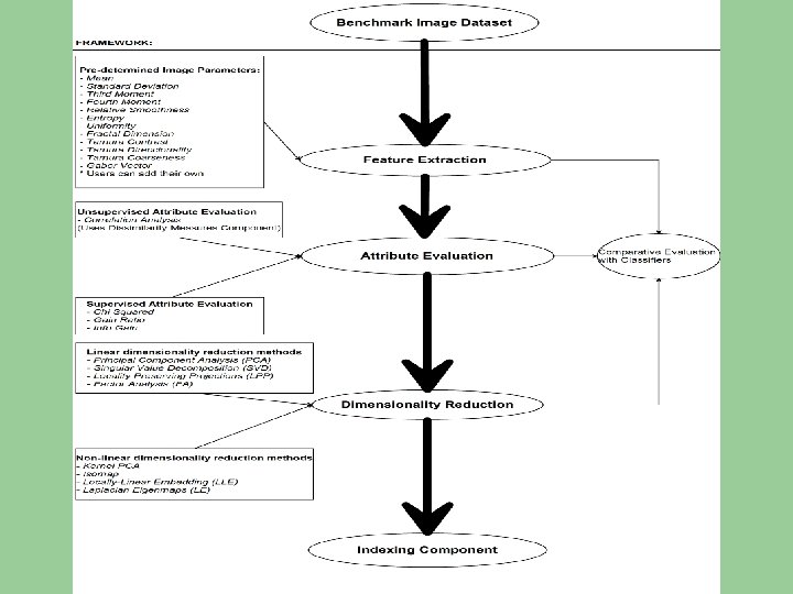
Framework Description

Feature Extraction
![Image Parameters Label Image parameter [29] P 1 Entropy P 2 Mean P 3](http://slidetodoc.com/presentation_image_h2/52d27061c44a65eca9b8f6eee8f2c719/image-22.jpg "Image Parameters Label Image parameter [29] P 1 Entropy P 2 Mean P 3")
Image Parameters Label Image parameter [29] P 1 Entropy P 2 Mean P 3 Standard Deviation P 4 3 rd Moment (skewness) P 5 4 th Moment (kurtosis) P 6 Uniformity P 7 Relative Smoothness (RS) P 8 Fractal Dimension [21] P 9 Tamura Directionality P 10 Tamura Contrast P 11 Tamura Coarseness P 12 Gabor Vector [17]

Image Segmentation / Feature Extraction 8 by 8 grid segmentation (128 x 128 pixels per cell) Image 1 - Cell 1, 1 Value Entropy 0. 1231 Mean 0. 2552 Standard Deviation 0. 1723 3 rd Moment (skewness) 0. 1873 4 th Moment (kurtosis) 0. 1825 Uniformity 0. 5671 Relative Smoothness (RS) 0. 1245 Fractal Dimension 0. 1525 Tamura Directionality 0. 2837 Tamura Contrast 0. 3645

Image Parameter Extraction Times for 1, 600 Images

Comparative Evaluation NB SVM C 4. 5 ADA C 4. 5 31. 65% 40. 45% 65. 60% 72. 41% Average classification accuracy with cell labeling Some of these results are part of the paper accepted for publication in the FLAIRS-23 conference (2010)

Attribute Evaluation

Motivation for this stage l By selecting the most relevant image parameters we will be able to save processing and storage costs for each parameter that we remove l SDO Image parameter vector will grow 6 Gigabytes per day
 b) Average correlation map for the Active Region class in")
Unsupervised Attribute Evaluation a) b) Average correlation map for the Active Region class in the one image as a query against: a) the same class scenario (intra-class correlation) ( 1 image vs. 199 images) b) other classes (inter-class correlation) scenario (1 image vs. 1, 400 images)
 b) MDS map for the Active Region class in the one")
Better Visualization? a) b) MDS map for the Active Region class in the one image as a query against: a) the same class scenario (intra-class correlation) ( 1 image vs. 199 images) b) other classes (inter-class correlation) scenario (1 image vs. 1, 400 images) Multidimensional Scaling (MDS) allows us to better visualize these correlations

Supervised Attribute Evaluation l Chi Squared l Gain Ratio l Info Gain User Extendable (WEKA has more than 15 other methods that the user can select)

Supervised Attribute Evaluation Chi Squared Info Gain Ratio Ranking Label 13322. 43 P 1 0. 624 P 9 0. 197 P 9 13142. 86 P 6 0. 606 P 6 0. 166 P 1 13104. 00 P 7 0. 605 P 7 0. 162 P 6 11686. 84 P 9 0. 599 P 1 0. 161 P 7 11646. 01 P 2 0. 544 P 4 0. 157 P 10 11504. 63 P 4 0. 532 P 5 0. 154 P 4 11274. 94 P 10 0. 525 P 10 0. 149 P 5 11226. 03 P 5 0. 490 P 2 0. 137 P 2 9040. 03 P 3 0. 398 P 3 0. 136 P 8 6624. 91 P 8 0. 381 P 8 0. 123 P 3

Experimental Set-up l Objective: 30% dimensionality reduction l Remove 3 parameters for each set of experiments Experiment Labels Exp 1 - All Parameters Exp 2 - Removing 8, 9, 10 Exp 3 - Removing 3, 6, 10 Exp 4 - Removing 3, 2, 5 Exp 5 - Removing 9, 6, 1 Exp 6 - Removing 8, 2, 5 Exp 7 - Removing 7, 6, 1

Attribute Evaluation – Preliminary Experimental Results Naïve Bayes SVM C 45 ADA C 45 Exp 1 31. 65% 40. 45% 65. 60 % Exp 2 28. 59% 34. 84% 59. 26% 63. 86% Exp 3 33. 23% 39. 50% 63. 55% 69. 49% Exp 4 30. 17% 34. 43% 53. 06% 57. 38% Exp 5 30. 25% 34. 14% 60. 17% 64. 96% Exp 6 29. 37% 35. 58% 56. 53% 61. 41% Exp 7 32. 72% 37. 89% 63. 50% 69. 32% 72. 41%

Attribute Evaluation - Preliminary Conclusions l Removal of some image parameters maintains comparable classification accuracy l Saving up to 30% of storage and processing costs l Paper: Accepted for publication in DICTA 2010 conference

Dimensionality Reduction

Motivation l By eliminating redundant dimensions we will be able to save retrieval and storage costs l In our case: 540 kilobytes per dimension per day, since we will have a 10, 240 dimensional image parameter vector per image (5. 27 GB per day)
 Singular Value Decomposition")
l Linear dimensionality reduction methods – – Principal Component Analysis (PCA) Singular Value Decomposition (SVD) Locality Preserving Projections (LPP) Factor Analysis (FA)
 Laplacian")
l Non-linear Dimensionality Reduction Methods – – Kernel PCA Isomap Locally-Linear Embedding (LLE) Laplacian Eigenmaps (LE)

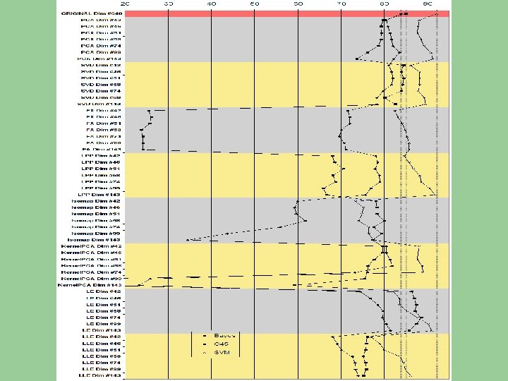
Experimental Set-up l We selected 67% of our data as the training set and an the remaining 33% for evaluation l Full Image Labeling l For comparative evaluation we utilize the number of components returned by standard PCA and SVD’s algorithms, setting up a variance threshold between 96 and 99% of the variance 96% 97% 98% 99% PCA 42 46 51 58 SVD 58 74 99 143

Dimensionality Reduction - Preliminary Experimental Results Average classification accuracy per method

Dimensionality Reduction - Preliminary Experimental Results Average classification accuracy per method

Dimensionality Reduction - Preliminary Experimental Results Average classification accuracy per number of generated dimensions

Dimensionality Reduction – Preliminary Conclusions l Selecting anywhere between 42 and 74 dimensions provided stable results l For our current benchmark dataset we can reduce around 90% from 640 dimensions we started with l For the SDO mission a 90% reduction would imply savings of up to 4. 74 Gigabytes per day (from 5. 27 Gigabytes of data per day) l Paper: Under Review

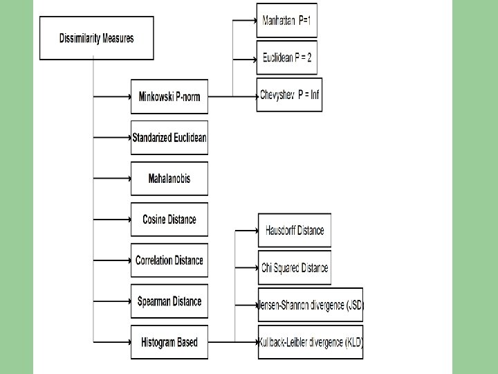
Dissimilarity Measures Component

Motivation for this stage l Literature reports very interesting results for different measures in different scenarios l The need to identify peculiar relationships between image parameters and different measures
![Dissimilarity Measures l 1) Euclidean distance [30]: Defined as the distance between two points](http://slidetodoc.com/presentation_image_h2/52d27061c44a65eca9b8f6eee8f2c719/image-47.jpg "Dissimilarity Measures l 1) Euclidean distance [30]: Defined as the distance between two points")
Dissimilarity Measures l 1) Euclidean distance [30]: Defined as the distance between two points give by the Pythagorean Theorem. Special case of the Minkowski metric where p=2. l 2) Standardized Euclidean distance [30]: Defined as the Euclidean distance calculated on standardized data, in this case standardized by the standard deviations.
![Dissimilarity Measures l 3) Mahalanobis distance [30]: Defined as the Euclidean distance normalized based](http://slidetodoc.com/presentation_image_h2/52d27061c44a65eca9b8f6eee8f2c719/image-48.jpg "Dissimilarity Measures l 3) Mahalanobis distance [30]: Defined as the Euclidean distance normalized based")
Dissimilarity Measures l 3) Mahalanobis distance [30]: Defined as the Euclidean distance normalized based on a covariance matrix to make the distance metric scale-invariant. l 4) City block distance [30]: Also known as Manhattan distance, it represents distance between points in a grid by examining the absolute differences between coordinates of a pair of objects. Special case of the Minkowski metric where p=1.
![Dissimilarity Measures l 5) Chebychev distance [30]: Measures distance assuming only the most significant](http://slidetodoc.com/presentation_image_h2/52d27061c44a65eca9b8f6eee8f2c719/image-49.jpg "Dissimilarity Measures l 5) Chebychev distance [30]: Measures distance assuming only the most significant")
Dissimilarity Measures l 5) Chebychev distance [30]: Measures distance assuming only the most significant dimension is relevant. Special case of the Minkowski metric where p = ∞. l 6) Cosine distance [26]: Measures the dissimilarity between two vectors by finding the cosine of the angle between them.
![Dissimilarity Measures l 7) Correlation distance [26]: Measures the dissimilarity of the sample correlation](http://slidetodoc.com/presentation_image_h2/52d27061c44a65eca9b8f6eee8f2c719/image-50.jpg "Dissimilarity Measures l 7) Correlation distance [26]: Measures the dissimilarity of the sample correlation")
Dissimilarity Measures l 7) Correlation distance [26]: Measures the dissimilarity of the sample correlation between points as sequences of values. l 8) Spearman distance [25]: Measures the dissimilarity of the sample’s Spearman rank [25] correlation between observations as sequences of values.
![Dissimilarity Measures l 9) Hausdorff Distance [17]: Intuitively defined as the maximum distance of](http://slidetodoc.com/presentation_image_h2/52d27061c44a65eca9b8f6eee8f2c719/image-51.jpg "Dissimilarity Measures l 9) Hausdorff Distance [17]: Intuitively defined as the maximum distance of")
Dissimilarity Measures l 9) Hausdorff Distance [17]: Intuitively defined as the maximum distance of a histogram to the nearest point in the other histogram. l 10 ) Jensen–Shannon divergence (JSD) [15]: Also known as total divergence to the average, Jensen–Shannon divergence is a symmetrized and smoothed version of the Kullback–Leibler divergence.
![Dissimilarity Measures l 11) distance [22]: Measures the likeliness of one histogram being drawn](http://slidetodoc.com/presentation_image_h2/52d27061c44a65eca9b8f6eee8f2c719/image-52.jpg "Dissimilarity Measures l 11) distance [22]: Measures the likeliness of one histogram being drawn")
Dissimilarity Measures l 11) distance [22]: Measures the likeliness of one histogram being drawn from another one. l 12) Kullback–Leibler divergence (KLD) [12]: Measures the difference between two histograms H and H’. Often intuited as a distance metric, the KL divergence is not a true metric since the KL divergence from H to H’ is not necessarily the same as the KL divergence from H’ to H.

Experimental Set-up l Full image labeling l Total of 130 dissimilarity matrices (13 measures, counting KLD H-H’ and H’-H, times a total of 10 different image parameters) l Classes of our benchmark are separated on the axes, each class fits every 200 units (images)

Experimental Set-up l Performed basic dimensionality reduction with MDS to take full advantage of dissimilarity matrices l Two test scenarios – 10 component threshold – 135 degree tangent threshold

Dissimilarity Matrices - Preliminary Experimental Results Plot of dissimilarity matrix for: Correlation measure with image parameter mean (Note: Low dissimilarity is solid blue, high dissimilarity is red)

Dissimilarity Matrices - Preliminary Experimental Results Plot of dissimilarity matrix for: JSD measure with image parameter mean (Note: Low dissimilarity is solid blue, high dissimilarity is red)

Dissimilarity Matrices - Preliminary Experimental Results Plot of dissimilarity matrix for: Chebychev measure with image parameter Relative Smoothness (Note: Low dissimilarity is solid blue, high dissimilarity is red)

10 Component Threshold Preliminary Experimental Results Explained Percentage of correctly classified instances for the 10 component Threshold – for Chebychev Measure

10 Component Threshold - Preliminary Experimental Results Percentage of correctly classified instances

Tangent Thresholding - Preliminary Experimental Results l Number of components to use indicated by the tangent thresholding method

Tangent Thresholding - Preliminary Experimental Results l Percentage of correctly classified instances for the tangent-based component threshold

Overall Classification - Preliminary Experimental Results l Top 5 classification results for 10 component limited and tangent thresholded dimensionality reduction experiments

Dissimilarity Measures Component Preliminary Conclusions l Some dissimilarity measures, allowed us to easily discern the dissimilarities between our images in our dataset and provided different levels of relevance between different image parameters l Application of different measures with different parameters is very domain specific l Paper: Accepted for publication in CIDU 2010 (Invited for submission to Best of CIDU 2010 issue of Statistical Analysis and Data Mining journal (the official journal of ASA))

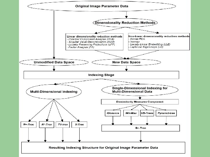
Indexing Component

Indexing and retrieval l Huge image parameter vector (up to 6 GB of growth per day), now what? l Huge repository that grows over 69, 000 images a day
 – TV-Trees (Apply")
Indexing approaches l Multi-Dimensional Indexing – R-trees (MBR’s – Overlapping problems) – TV-Trees (Apply dim. reduction, Telescope Vectors (dynamically reduced)) – X-Trees (minimizes overlapping w/ different algorithm and creation of super nodes)

Indexing approaches l Single-Dimensional Indexing for Multi. Dimensional Data – – i. Distance i. Min. Max UB-Trees Pyramid-trees

Motivation for this stage l Multi-dimensional indexing techniques not optimal for big number of dimensions l Current popularity of single dimensional approaches to high-dimensional data l Results have been very domain specific l Dimensionality reduced data spaces reduce index complexity

Objectives l High customization of indexing structure l Fast and simple retrieval l Obtaining the most efficient index by combination of elements
![References [1] R. Datta, D. Joshi, J. Li and J. Wang, “Image Retrieval: Ideas,](http://slidetodoc.com/presentation_image_h2/52d27061c44a65eca9b8f6eee8f2c719/image-70.jpg "References [1] R. Datta, D. Joshi, J. Li and J. Wang, “Image Retrieval: Ideas,")
References [1] R. Datta, D. Joshi, J. Li and J. Wang, “Image Retrieval: Ideas, Influences, and Trends of the New Age”, ACM Computing Surveys, vol. 40, no. 2, article 5, pp. 1 -60, 2008. [2] Y. Rui, T. S. Huang, S. Chang, “Image Retrieval: Current Techniques, Promising Directions, and Open Issues”. Journal of Visual Communication and Image Representation 10, pp. 39– 62, 1999. [3] H. Müller, N. Michoux, D. Bandon, A. Geissbuhler, “A review of content-based image retrieval systems in medical applications: clinical benefits and future directions”. International journal of medical informatics, Volume 73, pp. 1 -23, 2004 [4] Y. A Aslandogan, C. T Yu, “Techniques and systems for image and video retrieval” IEEE Transactions on Knowledge and Data Engineering, Vol: 11 1 , Jan. -Feb. 1999. [5] A. Yoshitaka, T. Ichikawa “A survey on content-based retrieval for multimedia databases” IEEE Transactions on Knowledge and Data Engineering, Vol: 11 1 , Jan. Feb. 1999. [6] T. Deselaers, D. Keysers, and H. Ney, "Features for Image Retrieval: An Experimental Comparison", Information Retrieval, Vol. 11, issue 2, The Netherlands, Springer, pp. 77 -107, 2008. [7] H. Müller, A. Rosset, J-P. Vallée, A. Geissbuhler, Comparing feature sets for content-based medical information retrieval. SPIE Medical Imaging, San Diego, CA, USA, February 2004. [8] S. Antani, L. R. Long, G. Thomas. "Content-Based Image Retrieval for Large Biomedical Image Archives" Proceedings of 11 th World Congress on Medical Informatics (MEDINFO) 2004 Imaging Informatics. September 7 -11 2004; San Francisco, CA, USA. 829 -33. 2004. [9] R. Lamb, “An Information Retrieval System For Images From The Trace Satellite, ” M. S. thesis, Dept. Comp. Sci. , Montana State Univ. , Bozeman, MT, 2008. [10] V. Zharkova, S. Ipson, A. Benkhalil and S. Zharkov, “Feature recognition in solar images, " Artif. Intell. Rev. , vol. 23, no. 3, pp. 209 -266. 2005. [11] M. Hall, E. Frank, G. Holmes, B. Pfahringer, P. Reutemann, I. H. Witten. “The WEKA Data Mining Software: An Update” SIGKDD Explorations, Volume 11, Issue 1, 2009 [12] K. Yang, J. Trewn. Multivariate Statistical Methods in Quality Management. Mc. Graw-Hill Professional; pp. 183 -185. 2004. [13] J. Lin. "Divergence measures based on the shannon entropy". IEEE Transactions on Information Theory 37 (1): pp. 145– 151. 2001. [14] S. Kullback, R. A. Leibler "On Information and Sufficiency". Annals of Mathematical Statistics 22 (1): pp. 79– 86. 1951. [15] J. Munkres. Topology (2 nd edition). Prentice Hall, pp 280 -281. 1999. [16] K. Pearson, "On lines and planes of closest fit to systems of points in space". Philosophical Magazine 2 (6) 1901, pp 559– 572. [17] M. Belkin and P. Niyogi. Laplacian Eigenmaps and spectral techniques for embedding and clustering. In Advances in Neural Information Processing Systems, volume 14, pp. 585– 591, Cambridge, MA, USA. The MIT Press. 2002. [18] L. K. Saul, K. Q. Weinberger, J. H. Ham, F. Sha, and D. D. Lee. Spectral methods for dimensionality reduction. In Semisupervised Learning, Cambridge, MA, USA, The MIT Press. 2006. [19] T. Etzold, A. Ulyanov, P. Argos. "SRS: information retrieval system for molecular biology data banks". Methods Enzymol. pp. 114– 128. 1999 [20] D. S. Raicu, J. D. Furst, D. Channin, D. H. Xu, & A. Kurani, "A Texture Dictionary for Human Organs Tissues' Classification", Proceedings of the 8 th World Multiconference on Systemics, Cybernetics and Informatics (SCI 2004), Orlando, USA, in July 18 -21, 2004.
![References [21] P. Korn, N. Sidiropoulos, C. Faloutsos, E. Siegel, and Z. Protopapas, "Fast](http://slidetodoc.com/presentation_image_h2/52d27061c44a65eca9b8f6eee8f2c719/image-71.jpg "References [21] P. Korn, N. Sidiropoulos, C. Faloutsos, E. Siegel, and Z. Protopapas, \"Fast")
References [21] P. Korn, N. Sidiropoulos, C. Faloutsos, E. Siegel, and Z. Protopapas, "Fast and effective retrieval of medical tumor shapes, " IEEE Transactions on Knowledge and Data Engineering, vol. 10, no. 6, pp. 889 -904. 1998. [22] J. M. Banda and R. Anrgyk “An Experimental Evaluation of Popular Image Parameters for Monochromatic Solar Image Categorization”. FLAIRS-23: Proceedings of the twenty-third international Florida Artificial Intelligence Research Society conference, Daytona Beach, Florida, USA, May 19– 21 2010. [23] Heliophysics Event Registry [Online] Available: http: //www. lmsal. com/~cheung/hpkb/index. html [Accessed: Sep 24, 2010] [24] TRACE On-line (TRACE) [Online], Available: http: // trace. lmsal. com/. [Accessed: Sep 29, 2010] [25] TRACE Data set (MSU) [Online], Available: http: //www. cs. montana. edu/angryk/SDO/data/TRACEbenchmark / [Accessed: Sep 29, 2010] [26] J. M Banda and R. Angryk “On the effectiveness of fuzzy clustering as a data discretization technique for large-scale classification of solar images” Proceedings of the 18 th IEEE International Conference on Fuzzy Systems (FUZZ-IEEE ’ 09), Jeju Island, Korea, August 2009, pp. 2019 -2024. 2009. [27] A. Pronobis, B. Caputo, P. Jensfelt, and H. I. Christensen. “A discriminative approach to robust visual place recognition”. In Proceedings of the IEEE/RSJ International Conference on Intelligent Robots and Systems (IROS 06), Beijing, China, 2006. [28] The INDECS Database [Online], Available: http: //cogvis. nada. kth. se/INDECS/ [Accessed: Sep 29, 2010] [29] W. Hersh, H. Müller, J. Kalpathy-Cramer, E. Kim, X. Zhou, “The consolidated Image. CLEFmed Medical Image Retrieval Task Test Collection”, Journal of Digital Imaging, volume 22(6), 2009, pp 648 -655. [30] Cross Language Evaluation Forum [Online], Available: http: //www. clef-campaign. org/ [Accessed: Sep 29, 2010] [31] Image CLEF – Image Retrieval in CLEF, Available: http: //www. imageclef. org/2010/medical [Accessed: Sep 29, 2010] [32] V. Zharkova and V. Schetinin, “Filament recognition in solar images with the neural network technique, " Solar Physics, vol. V 228, no. 1, 2005, pp. 137 -148. 2005. [33] V. Delouille, J. Patoul, J. Hochedez, L. Jacques and J. P. Antoine , “Wavelet spectrum analysis of eit/soho images, " Solar Physics, vol. V 228, no. 1, 2005, pp. 301321. 2005. [34] A. Irbah, M. Bouzaria, L. Lakhal, R. Moussaoui, J. Borgnino, F. Laclare and C. Delmas, “Feature extraction from solar images using wavelet transform: image cleaning for applications to solar astrolabe experiment. ” Solar Physics, Volume 185, Number 2, April 1999 , pp. 255 -273(19). 1999. [35] K. Bojar and M. Nieniewski. “Modelling the spectrum of the fourier transform of the texture in the solar EIT images”. MG&V 15, 3, pp. 285 -295. 2006. [36] S. Christe, I. G. Hannah, S. Krucker, J. Mc. Tiernan, and R. P. Lin. “RHESSI Microflare Statistics. I. Flare-Finding and Frequency Distributions”. Ap. J, 677 pp. 1385 – 1394. 2008. [37] P. N. Bernasconi, D. M. Rust, and D. Hakim. “Advanced Automated Solar Filament Detection And Characterization Code: Description, Performance, And Results”. Sol. Phys. , 228. pp. 97– 117, 2005. [38] A. Savcheva, J. Cirtain, E. E. Deluca, L. L. Lundquist, L. Golub, M. Weber, M. Shimojo, K. Shibasaki, T. Sakao, N. Narukage, S. Tsuneta, and R. Kano. “A Study of Polar Jet Parameters Based on Hinode XRT Observations”. Publ. Astron. Soc. Japan, 59: 771–+. 2007. [39] I. De Moortel and R. T. J. Mc. Ateer. “Waves and wavelets: An automated detection technique for solar oscillations”. Sol. Phys. , 223. pp. 1– 2. 2004. [40] R. T. J. Mc. Ateer, P. T. Gallagher, D. S. Bloomfield, D. R. Williams, M. Mathioudakis, and F. P. Keenan. “Ultraviolet Oscillations in the Chromosphere of the Quiet Sun”. Ap. J, 602, pp. 436– 445. 2004.
![References [41] S. Kulkarni, B. Verma, "Fuzzy Logic Based Texture Queries for CBIR, "](http://slidetodoc.com/presentation_image_h2/52d27061c44a65eca9b8f6eee8f2c719/image-72.jpg "References [41] S. Kulkarni, B. Verma, \"Fuzzy Logic Based Texture Queries for CBIR, \"")
References [41] S. Kulkarni, B. Verma, "Fuzzy Logic Based Texture Queries for CBIR, " Fifth International Conference on Computational Intelligence and Multimedia Applications (ICCIMA'03), pp. 223, 2003 [42] H Lin, C Chiu, and S. Yang, “ Lin. Star texture: a fuzzy logic CBIR system for textures”, In Proceedings of the Ninth ACM international Conference on Multimedia (Ottawa, Canada). MULTIMEDIA '01, vol. 9. ACM, New York, NY, pp 499 -501. 2001. [43] S. Thumfart, W. Heidl, J. Scharinger, and C. Eitzinger. “A Quantitative Evaluation of Texture Feature Robustness and Interpolation Behaviour”. In Proceedings of the 13 th international Conference on Computer Analysis of Images and Patterns. 2009. [44] J. Muwei, L. Lei, G. Feng, "Texture Image Classification Using Perceptual Texture Features and Gabor Wavelet Features, " Asia-Pacific Conference on Information Processing vol. 2, pp. 55 -58, 2009. [45] E. Cernadas, P. Carriön, P. Rodriguez, E. Muriel, and T. Antequera. “Analyzing magnetic resonance images of Iberian pork loin to predict its sensorial characteristics” Comput. Vis. Image Underst. 98, 2 pp. 345 -361. 2005. [46] S. S. Holalu and K. Arumugam “Breast Tissue Classification Using Statistical Feature Extraction Of Mammograms”, Medical Imaging and Information Sciences, Vol. 23 No. 3, pp. 105 -107. 2006 [47] S. T. Wong, H. Leung, and H. H. Ip, “Model-based analysis of Chinese calligraphy images” Comput. Vis. Image Underst. 109, 1 (Jan. 2008), pp. 69 -85. 2008. [48] V. Devendran, T. Hemalatha, W. Amitabh "SVM Based Hybrid Moment Features for Natural Scene Categorization, " International Conference on Computational Science and Engineering vol. 1, pp. 356 -361, 2009. [49] B. B. Chaudhuri, Nirupam Sarkar, "Texture Segmentation Using Fractal Dimension, " IEEE Transactions on Pattern Analysis and Machine Intelligence, vol. 17, no. 1, pp. 72 -77, Jan. 1995 [51] C. Wen-lun, S. Zhong-ke, F. Jian, "Traffic Image Classification Method Based on Fractal Dimension, " IEEE International Conference on Cognitive Informatics Vol. 2, pp. 903 -907, 2006. [52] A. P Pentland, “Fractal-based description of natural scenes’, IEEE Trans. on Pattern Analysis and Machine Intelligence, 6 pp. 661 -674, 1984. [53] H. F. Jelinek, D. J. Cornforth, A. J. Roberts, G. Landini, P. Bourke, and A. Iorio, “Image processing of finite size rat retinal ganglion cells using multifractal and local connected fractal analysis”, In 17 th Australian Joint Conference on Artificial Intelligence, volume 3339 of Lecture Notes in Computer Science, pages 961 --966. Springer--Verlag Heidelberg, 2004 [54] M. Schroeder. Fractals, Chaos, Power Laws: Minutes from an Infinite Paradise. New York: W. H. Freeman, pp. 41 -45, 1991. [55] H. Tamura, S. Mori, T. Yamawaki. “Textural Features Corresponding to Visual Perception”. IEEE Transaction on Systems, Man, and Cybernetics 8(6): pp. 460– 472. 1978. [56] R. M Haralick, K. Shanmugam and I. Dinstein, “Textural Features For Image Classification, ” IEEE Transactions on Systems, Man, and Cybernetics, Volume: SMC 3, No. 6, pp 610 - 621. 1978. [57] N. Vasconcelos, M. Vasconcelos. “Scalable Discriminant Feature Selection for Image Retrieval and Recognition”. In CVPR 2004. (Washington, DC 2004), pp. 770 – 775. 2004. [58] M. Schroeder. “Fractals, Chaos, Power Laws: Minutes from an Infinite Paradise”. (W. H. Freeman, New York 1991), pp. 41 -45. 1991. [59] S. Kullback, and R. A. Leibler. “On Information and Sufficiency”. Annals of Mathematical Statistics 22, pp. 79– 86. 1951. [60] J. R. Quinlan. “Induction of decision trees”. Machine Learning, pp. 81 -106, 1986.
![References [61] G. D Guo, A. K. Jain, W. Y Ma, H. J Zhang,](http://slidetodoc.com/presentation_image_h2/52d27061c44a65eca9b8f6eee8f2c719/image-73.jpg "References [61] G. D Guo, A. K. Jain, W. Y Ma, H. J Zhang,")
References [61] G. D Guo, A. K. Jain, W. Y Ma, H. J Zhang, et. al, "Learning similarity measure for natural image retrieval with relevance feedback". IEEE Transactions on Neural Networks. Volume 13 (4). pp. 811 -820, 2002. [62] R. Lam, H. Ip, K. Cheung, L. Tang, R. Hanka, "Similarity Measures for Histological Image Retrieval, " 15 th International Conference on Pattern Recognition (ICPR'00) - Volume 2. pp. 2295. 2000. [63] T. Ojala, M. Pietikainen, and D. Harwood. A comparative study of texture measures with classification based feature distributions. Pattern Recognition, 29(1). pp. 51– 59. 1996. [64] P. -N. Tan, M. Steinbach & V. Kumar, "Introduction to Data Mining", Addison-Wesley pp. 500, 2005. [65] C. Spearman, "The proof and measurement of association between two things" Amer. J. Psychol. , V 15. pp. 72– 101. 1904 [66] P. Moravec, and V. Snasel, “Dimension reduction methods for image retrieval”. In Proceedings of the Sixth international Conference on intelligent Systems Design and Applications - Volume 02 (October 16 - 18, 2006). ISDA. IEEE Computer Society, Washington, DC, pp. 1055 -1060. 2006. [67] J. Ye, R. Janardan, and Q. Li, “GPCA: an efficient dimension reduction scheme for image compression and retrieval”. In Proceedings of the Tenth ACM SIGKDD international Conference on Knowledge Discovery and Data Mining (Seattle, WA, USA, August 22 - 25, 2004). KDD '04. ACM, New York, NY, pp. 354 -363. 2004. [68] E. Bingham, and H. Mannila, “Random projection in dimensionality reduction: applications to image and text data”. In Proceedings of the Seventh ACM SIGKDD international Conference on Knowledge Discovery and Data Mining (San Francisco, California, August 26 - 29, 2001). KDD '01. ACM, New York, NY, pp. 245250. 2001. [69] A. Antoniadis, S. Lambert- Lacroix, F. Leblanc, F. “Effective dimension reduction methods for tumor classification using gene expression data”. Bioinformatics, vol 19, pp. 563– 570. 2003. [70] J. Harsanyi and C. -I Chang, “Hyperspectral image classification and dimensionality reduction: An orthogonal subspace projection approach, ” IEEE Trans. Geosci. Remote Sensing, vol. 32, pp. 779– 785. 1994. [71] L. J. P. van der Maaten, E. O. Postma, and H. J. van den Herik. “Dimensionality reduction: a comparative review”. Tilburg University Technical Report, Ti. CC-TR 2009 -005, 2009. [72] C. Eckart, G. Young, "The approximation of one matrix by another of lower rank", Psychometrika 1 (3), pp 211– 218. 1936. [73] X. He and P. Niyogi, “Locality Preserving Projections, ” Proc. Conf. Advances in Neural Information Processing Systems, V 16. pp 153 -160. 2003. [74] D. N. Lawley, and A. E. Maxwell. “Factor analysis as a statistical method”. 2 nd Ed. New York: American Elsevier Publishing Co. , 1971. [75] B. Schölkopf, A. Smola, and K. -R. Muller. “Kernel principal component analysis”. In Proceedings ICANN 97, Springer Lecture Notes in Computer Science, pp. 583, 1997. [76] J. B. Tenenbaum, V. de Silva, and J. C. Langford. ” A global geometric framework for nonlinear dimensionality reduction”. Science, 290(5500) pp 2319– 2323, 2000. [77] D. Comer. “Ubiquitous B-Tree. ”, ACM Comput. Surv. 11, 2 (Jun. 1979), pp. 121 -137. 1979 [78] C. Yu, B. C. Ooi, K. Tan and H. V. Jagadish. “Indexing the distance: an efficient method to KNN processing”, Proceedings of the 27 st international conference on Very large data bases, Roma, Italy, 421 -430, 2001. [79] H. V. Jagadish, B. C. Ooi, K. Tan, C. Yu and R. Zhang “ i. Distance: An Adaptive B+-tree Based Indexing Method for Nearest Neighbor Search”, ACM Transactions on Data Base Systems (ACM TODS), 30, 2, pp. 364 -397, 2005. [80] B. C. Ooi, K. L. Tan, C. Yu, and S. Bressan. “Indexing the edge: a simple and yet efficient approach to high-dimensional indexing”. In Proc. 18 th ACM SIGACTSIGMOD-SIGART Symposium on Principles of Database Systems, pp. 166 -174. 2000.
![References [81] V. Markl. “MISTRAL: Processing Relational Queries using a Multidimensional Access Technique”. Ph.](http://slidetodoc.com/presentation_image_h2/52d27061c44a65eca9b8f6eee8f2c719/image-74.jpg "References [81] V. Markl. “MISTRAL: Processing Relational Queries using a Multidimensional Access Technique”. Ph.")
References [81] V. Markl. “MISTRAL: Processing Relational Queries using a Multidimensional Access Technique”. Ph. D Thesis. Der Technischen Universität München. 1999. [82] R. Zhang, P. Kalnis, B. C. Ooi, K. Tan. “Generalized Multi-dimensional Data Mapping and Query Processing”. ACM Transactions on Data Base Systems (TODS), 30(3): pp. 661 -697, 2005. [83] S. Berchtold, C. Böhm, and H. Kriegal. “The pyramid-technique: towards breaking the curse of dimensionality”. In Proceedings of the 1998 ACM SIGMOD international Conference on Management of Data (Seattle, Washington, United States, June 01 - 04, 1998). SIGMOD '98. ACM, New York, NY, pp. 142 -153. 1998. [84] F. Ramsak, M. Volker, R. Fenk, M. Zirkel, K. Elhardt, R. Bayer. "Integrating the UB-tree into a Database System Kernel". 26 th International Conference on Very Large Data Bases. pp. 263– 272. 2000. [85] S. Berchtold, C. Böhm, H. P. Kriegel. “The Pyramid-Technique: Towards indexing beyond the Curse of Dimensionality”, Proc. ACM SIGMOD Int. Conf. on Management of Data, Seattle, pp. 142 -153, 1998. [86] A. Guttman. “R-trees: A Dynamic Index Structure for Spatial Searching”, Proc. ACM SIGMOD Int. Conf. on Management of Data, Boston, MA, pp. 47 -57. 1984. [87] S. Berchtold, D. Keim, H. P. Kriegel. “The X-Tree: An Index Structure for High-Dimensional Data”, 22 nd Conf. on Very Large Databases, Bombay, India, pp. 28 -39. 1996. [88] T. Sellis, N. Roussopoulos, C. Faloutsos. “The R+-Tree: A Dynamic Index for Multi-Dimensional Objects”, Proc. 13 th Int. Conf. on Very Large Databases, Brighton, England, pp. 507 -518. 1987. [89] N. Beckmann, H. P. Kriegel, R. Schneider, B. Seeger. “The R*-tree: An Efficient and Robust Access Method for Points and Rectangles”, Proc. ACM SIGMOD Int. Conf. on Management of Data, Atlantic City, NJ, pp. 322 -331. 1990. [90] D. A White, R. Jain. “Similarity indexing with the SS-tree”, Proc. 12 th Int. Conf on Data Engineering, New Orleans, LA, 1996. [91] K. Lin, H. V. Jagadish, C. Faloutsos. “The TV-Tree: An Index Structure for High-Dimensional Data”, VLDB Journal, Vol. 3, pp. 517542, 1995. [92] A. Shahrokni. “Texture Boundary Detection for Real-Time Tracking” Computer Vision - ECCV 2004. pp. 566 -577. 2004.

Appendix: SDO Solar Images

Image Segmentation / Feature Extraction 8 by 8 grid segmentation (128 x 128 pixels per cell) Image 1 - Cell 1, 1 Value Entropy 0. 1231 Mean 0. 2552 Standard Deviation 0. 1723 3 rd Moment (skewness) 0. 1873 4 th Moment (kurtosis) 0. 1825 Uniformity 0. 5671 Relative Smoothness (RS) 0. 1245 Fractal Dimension 0. 1525 Tamura Directionality 0. 2837 Tamura Contrast 0. 3645
- Slides: 76