Fractional Cascading and Its Applications G S Lueker

Fractional Cascading and Its Applications • G. S. Lueker. A data structure for orthogonal range queries. In Proc. 19 th annu. IEEE Sympos. Found. Comput. Sci. , pages 28 -34, 1978. • D. E. Willard. Predicate-oriented database search algorithms. Ph. D. thesis, Aiken Comput. Lab. , Harvard Univ. , Cambridge, MA, 1978, Report TR-20 -78. • B. Chazelle, L. J. Guibas: Fractional Cascading: I. A Data Structuring Technique. Algorithmica 1(2): 133 -162 (1986) • B. Chazelle, L. J. Guibas: Fractional Cascading: II. Applications. Algorithmica 1(2): 163 -191 (1986) Slides by Dror Aiger

What is Fractional Cascading? • A technique to speed up a sequence of binary searches for the same value in a sequence of related data structures. • The first binary search in the sequence takes a logarithmic time, but successive searches in the sequence are faster.

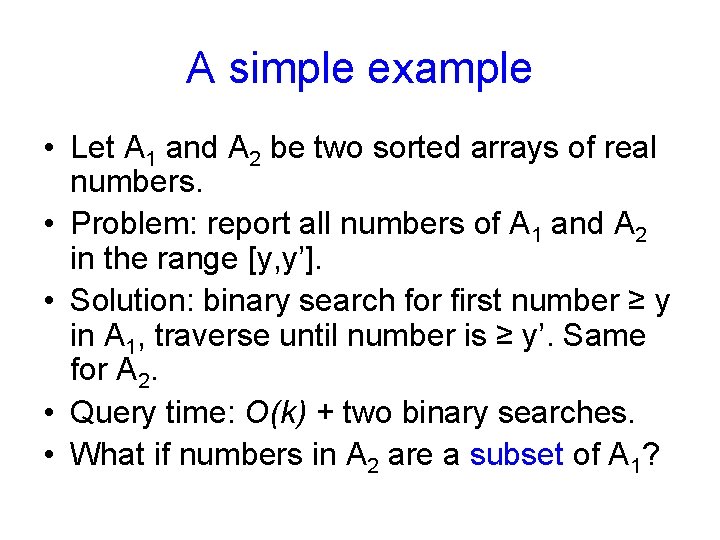
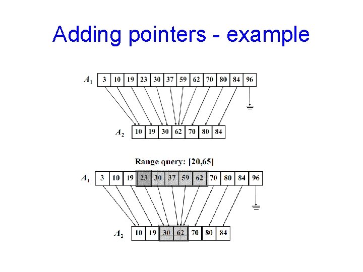
A simple example • Let A 1 and A 2 be two sorted arrays of real numbers. • Problem: report all numbers of A 1 and A 2 in the range [y, y’]. • Solution: binary search for first number ≥ y in A 1, traverse until number is ≥ y’. Same for A 2. • Query time: O(k) + two binary searches. • What if numbers in A 2 are a subset of A 1?

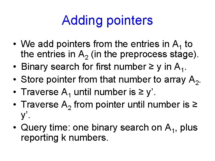
Adding pointers • We add pointers from the entries in A 1 to the entries in A 2 (in the preprocess stage). • Binary search for first number ≥ y in A 1. • Store pointer from that number to array A 2. • Traverse A 1 until number is ≥ y’. • Traverse A 2 from pointer until number is ≥ y’. • Query time: one binary search on A 1, plus reporting k numbers.

Adding pointers - example

Application in Range Searching • In the plane the query time of range trees is O(log 2(n)+k). • Can we do better? • Yes, we can obtain O(log(n)+k) query time with fractional cascading.

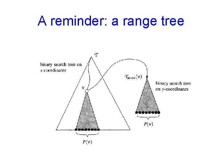
A reminder: a range tree

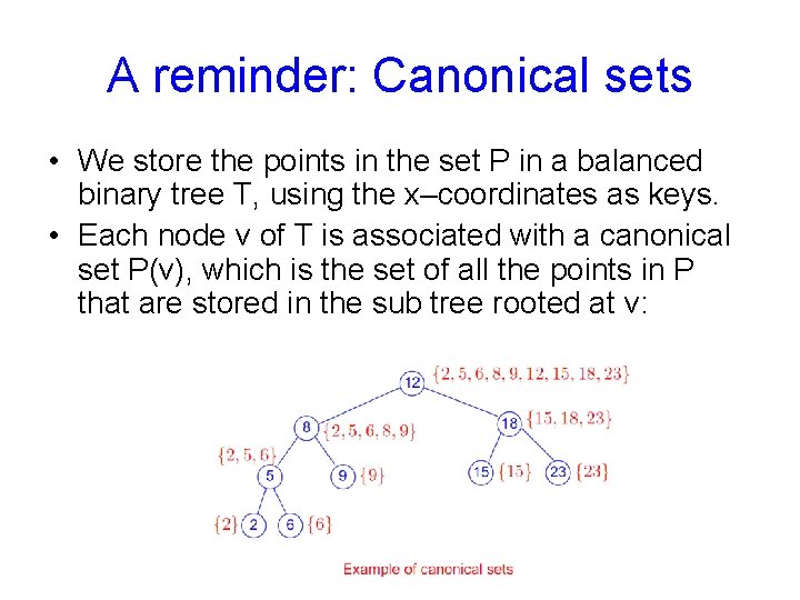
A reminder: Canonical sets • We store the points in the set P in a balanced binary tree T, using the x–coordinates as keys. • Each node v of T is associated with a canonical set P(v), which is the set of all the points in P that are stored in the sub tree rooted at v:

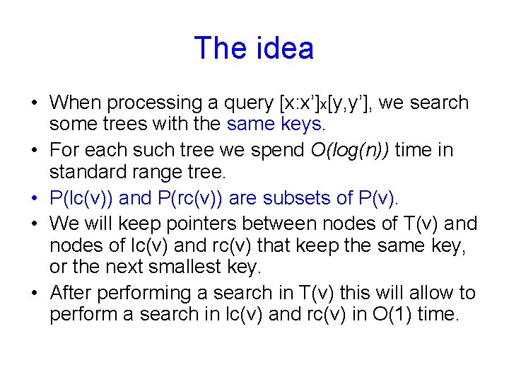
The idea • When processing a query [x: x’]x[y, y’], we search some trees with the same keys. • For each such tree we spend O(log(n)) time in standard range tree. • P(lc(v)) and P(rc(v)) are subsets of P(v). • We will keep pointers between nodes of T(v) and nodes of lc(v) and rc(v) that keep the same key, or the next smallest key. • After performing a search in T(v) this will allow to perform a search in lc(v) and rc(v) in O(1) time.

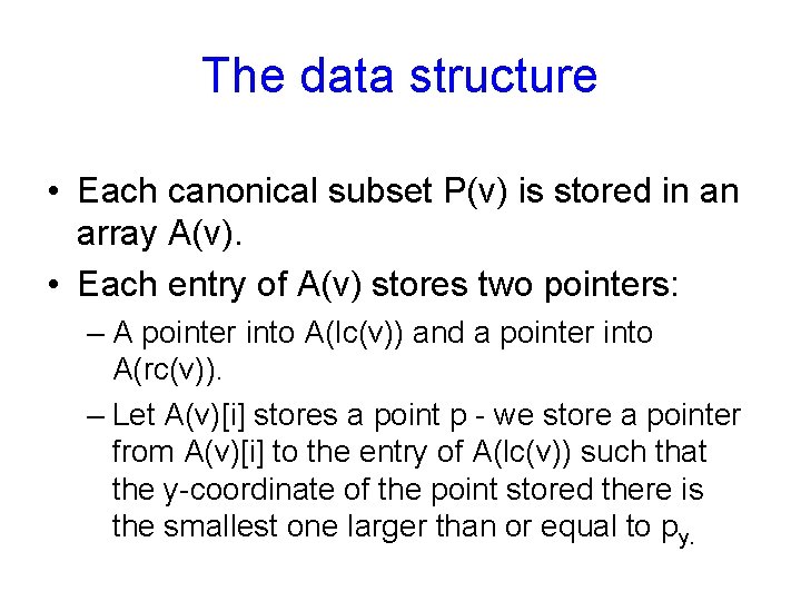
The data structure • Each canonical subset P(v) is stored in an array A(v). • Each entry of A(v) stores two pointers: – A pointer into A(lc(v)) and a pointer into A(rc(v)). – Let A(v)[i] stores a point p - we store a pointer from A(v)[i] to the entry of A(lc(v)) such that the y-coordinate of the point stored there is the smallest one larger than or equal to py.

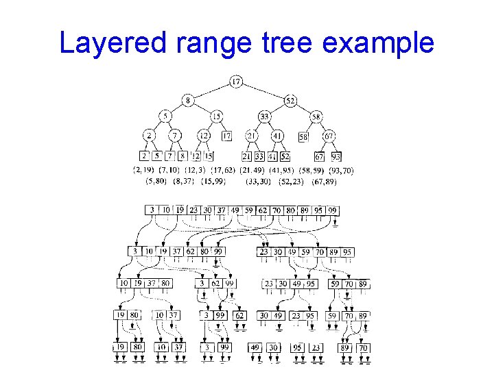
Layered range tree example

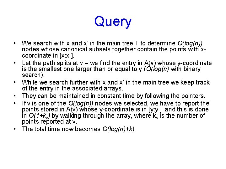
Query • We search with x and x’ in the main tree T to determine O(log(n)) nodes whose canonical subsets together contain the points with xcoordinate in [x: x’]. • Let the path splits at v – we find the entry in A(v) whose y-coordinate is the smallest one larger than or equal to y (O(log(n) with binary search). • While we search further with x and x’ in the main tree we keep track of the entry in the associated arrays. • They can be maintained in constant time by following the pointers. • If v is one of the O(log(n)) nodes we selected, we have to report the points stored in A(v) whose y-coordinate is in [y: y’] and this is done in O(1+kv) by walking through the array, where kv is the number of points reported at v. • The total time now becomes O(log(n)+k)

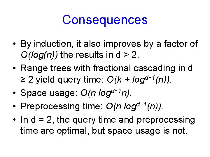
Consequences • By induction, it also improves by a factor of O(log(n)) the results in d > 2. • Range trees with fractional cascading in d ≥ 2 yield query time: O(k + logd− 1(n)). • Space usage: O(n logd− 1 n). • Preprocessing time: O(n logd− 1(n)). • In d = 2, the query time and preprocessing time are optimal, but space usage is not.

Another application • Intersecting a polygonal path with a line • CG 86 Bernard Chazelle, Leonidas J. Guibas: Fractional Cascading: II. Applications. Algorithmica 1(2): 163 -191 (1986)

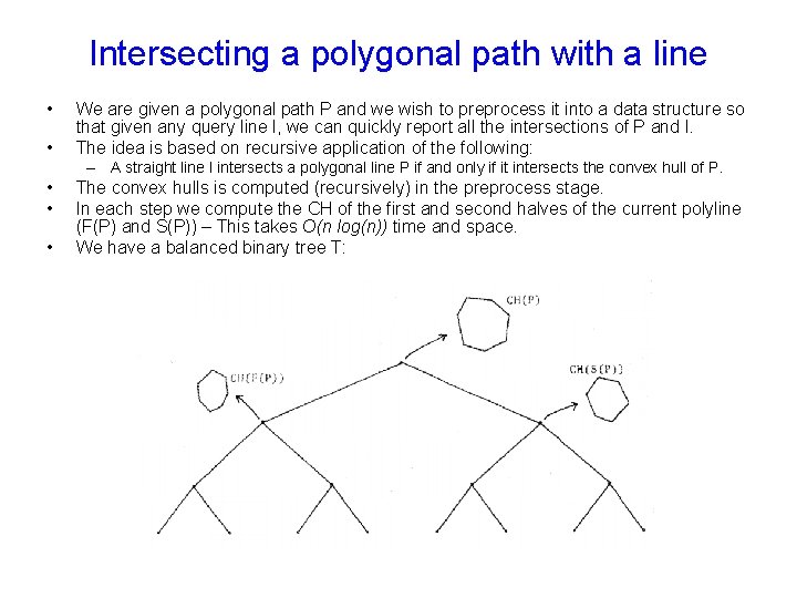
Intersecting a polygonal path with a line • • We are given a polygonal path P and we wish to preprocess it into a data structure so that given any query line l, we can quickly report all the intersections of P and l. The idea is based on recursive application of the following: – A straight line l intersects a polygonal line P if and only if it intersects the convex hull of P. • • • The convex hulls is computed (recursively) in the preprocess stage. In each step we compute the CH of the first and second halves of the current polyline (F(P) and S(P)) – This takes O(n log(n)) time and space. We have a balanced binary tree T:

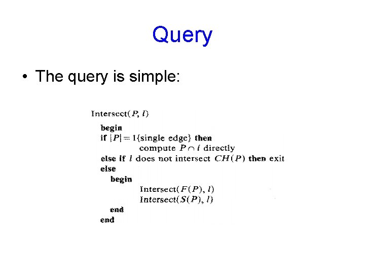
Query • The query is simple:

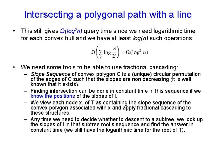
Intersecting a polygonal path with a line • This still gives Ω(log 2 n) query time since we need logarithmic time for each convex hull and we have at least log(n) such operations: • We need some tools to be able to use fractional cascading: – Slope Sequence of convex polygon C is a (unique) circular permutation of the edges of C such that the slopes are non decreasing (it is well known that it exists). – Finding intersection can be done in constant time in this sequence if we know the positions of the slopes of l. – We view each node x, of T as containing the slope sequence of the convex polygon associated with x and apply fractional cascading to these structures. – Any time we need to decide whether to descent to a subtree, we look up the slopes of l in that subtree root’s sequence and find the answer in constant time (we still have the logarithmic time for the root of T).

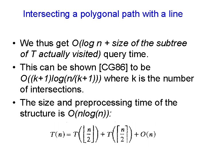
Intersecting a polygonal path with a line • We thus get O(log n + size of the subtree of T actually visited) query time. • This can be shown [CG 86] to be O((k+1)log(n/(k+1))) where k is the number of intersections. • The size and preprocessing time of the structure is O(nlog(n)):