Fourier Transform Insights and Techniques Synthesis Imaging School

Fourier Transform Insights and Techniques Synthesis Imaging School -- Narrabri, Sept. 2014 John Dickey University of Tasmania Including slides from Bob Watson

Outline 1. • • • One dimensional functions Fourier Series equations and examples Fourier Transform examples and principles Deconvolution and aliasing 2. Two dimensional functions • deconvolution • Combining single-dish and interferometer data Reference: The Fourier Transform and its Applications, R. N. Bracewell (John Wiley)

Statement of Fourier’s Theorem Suitable periodic functions, with a period of 2 p, may be represented as (called a Fourier series) series

Here The word “suitable” covers most functions you meet in physics

Complex form of Fourier’s Theorem Suitable periodic functions, with a period of 2 p, may be represented as where j = √-1 and

Triangular wave h -p p q

Triangular wave First 3 series terms: Waves: 5

Triangular wave Sum of first 2 terms: Waves: 5

Triangular wave Sum of first 3 terms: Waves: 5

Triangular wave Sum of first 5 terms: Waves: 5

Triangular wave Sum of first 10 terms: Waves: 5

Triangular wave All partial series sums up to 20 terms:

Half-wave rectifier h -p p q

Half-wave rectifier First 3 series terms: Waves: 5

Half-wave rectifier Sum of first 2 terms: Waves: 5

Half-wave rectifier Sum of first 3 terms: Waves: 5

Half-wave rectifier Sum of first 5 terms: Waves: 5

Half-wave rectifier Sum of first 10 terms: Waves: 5

Even square wave h -p p q

Even square wave First 3 series terms: Waves: 5

Even square wave Sum of first 2 terms: Waves: 5

Even square wave Sum of first 3 terms: Waves: 5

Even square wave Sum of first 5 terms: Waves: 5

Even square wave Sum of first 10 terms: Gibbs’ phenomenon Waves: 5

The Fourier Series Spectrum: Even square wave h -p q p a 1 = 4 h/p an a 1/5 -a 1/3 1 2 3 4 n 5

Example: Odd square wave h q -p p b 1 = 4 h/p b 1/3 bn b 1/5 n 1 2 3 4 5

Spectra for complex transform coefficients

-5 w 1 -3 w 1 -w 1 3 w 1 5 w 1 w Waves: 5

Temporally periodic case If we have a function f(t) , with temporal period T , which we wish to express as a Fourier series, then change our f(q) series using

So the Fourier series for f(t) = where Waves: 5

T is the fundamental period of f(t) and w 1 = 2 p/T is the fundamental angular frequency

Using w 1: f(t) = where Waves: 5

The corresponding complex form of f(t) in terms of w 1 is where

Taking T® ¥ in the complex form and substitute

Hence As T ® ¥

F(w) gives the continuous spectrum of real and imaginary parts (or amplitude and phase) that must be present to faithfully represent f(t) over an infinite interval.

-5 w 1 -3 w 1 -w 1 3 w 1 5 w 1 w Waves: 5

Fourier transform visualization w Waves: 5

FOURIER TRANSFORM DERIVATIONS Example 1: The rectangular or “slit” function f(t) h t -(1/2) t +(1/2) t

Derivation:

Thus F(w) has the form

Thus F(w) has the form F(w) -2 p +2 p -p + p -4 p/t +4 p/t -2 p/t +2 p/t Waves: 2 w

Example 2: Dirac delta-function f(t) h t ( By definition h-1 )

Derivation: Take the rectangular pulse of Example 1 and let t = h-1 Since first zero is at Then F(w) = 1 (constant for all w).

Note: 1. F(w) is again real and even, as expected for an even f(t) F(w) 1 w

Example 3: The Gauss function f(t) h s t h e-1/2

Derivation: Convert this to the form e- s 2 by the change of variables

Hence and since we have i. e. If f(t) is Gaussian with [h , s] then F(w) is Gaussian with [h(2 p)1/2 s , s -1]

PROPERTIES OF FOURIER TRANSFORMS Fourier transforms are sometimes of use in physics due to their direct physical interpretation (see later), but often their usefulness is more indirect

In particular, a great usefulness comes from their help in solving awkward differential equations Here we list several general transform properties of benefit in this and other contexts (Note that these properties are listed here without proofs Most proofs follow from the defining equations)

1. Linearity If then

2. Scale change If then Thus compressing a time function expands its spectrum in frequency and vice-versa

This expresses the idea of “Time ´ Bandwidth” invariance and is demonstrating in a general way the Bandwidth Theorem (i. e Dw. Dt ~ 2 p )

3. Delay and modulation If then

Thus : . . . delaying a time function f(t) simply adds a linear phase (-wt 0) to the original F(w) phase. . . modulating f(t) by ejw 0 t shifts the spectrum by w 0

Similarly, if one modulates by the real function cos(wot) we have Thus this real modulation gives a spectrum which is the average of two copies of the original form, one shifted by +w 0 and the other by -w 0

i. e. if f(t) transforms to w then [ cos(wot) f(t) ] transforms to -w 0 + w 0 w

4. Differentiation and integration If then

Thus taking the transform reduces differentiation and integration to the simpler operations of multiplication or division by jw in the frequency domain. Then finding the inverse transform gives the final result in the time domain This is analogous to the taking of logarithms to reduce “ ´ and ¸ ” to the simpler operations of “ + and - ”. In that case finding the anti-log gave the final result

5. Multiplication and convolution If then

Thus : . . . a product of functions has a transform that is the convolution of the individual transforms. . . conversely if you convolve functions you multiply their individual transforms

The delta function is the indentity operation for convolution:

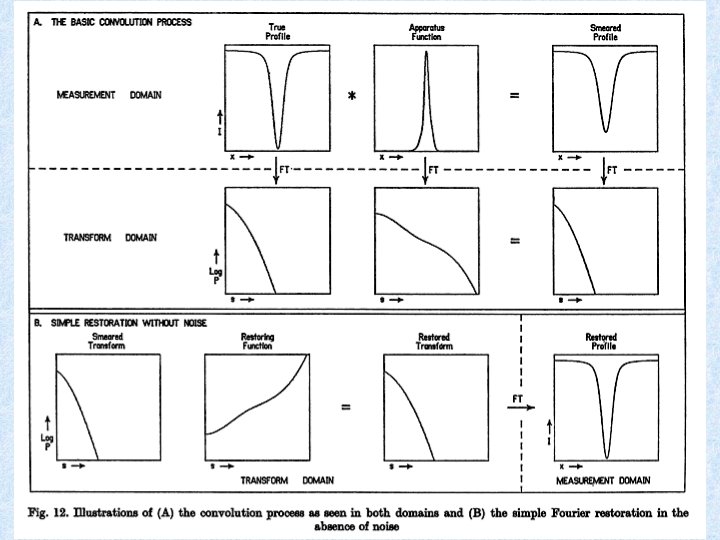
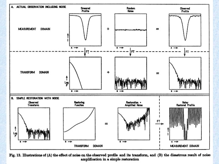
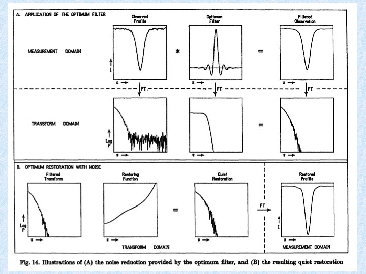
Next: A nicely illustrated example from an old paper by Brault and White (1971 Astron. & Astrophys. 13, 169). • • sampling theorem aliasing apodizing deconvolution

A continuous data function and its Fourier Transform.

Sampling (digitizing) the continuous function at different intervals.

After removing the mean, multiply by an apodizing or masking function to eliminate the discontinuity between the two ends.

Two Dimensional Fourier Transforms For a function of two dimensions, the Fourier Transform is done by transforming in each dimension separately.

Example : Ponte Vecchio in Florence… real imag

Example : Ponte Vecchio in Florence… data compressed by 4 : real imag

Example : Ponte Vecchio in Florence… (raw image 512 x 512) saving 16 x 16 pixels in the centre of transform saving 32 x 32 saving 64 x 64 saving 128 x 128

Convolving the image with a Gaussian:

Convolving the image with a Gaussian: Deconvolution with noise floors:

How can we get from here back to here? Most of the rest of the workshop will describe how to optimize the image making process.

Parkes Compact Array Combined data see Mc. Clure-Griffiths et al. 2000 and Stanimirovic 1999

Aperture or uv plane Image or lm plane Aperture synthesis mapping Single dish mapping

Conclusions: • • To understand aperture synthesis and interferometry in general review your Fourier transforms. Understanding the telescope and how it samples the sky requires visualization of the uv plane sampling function. Improving images by “deconvolution” of unsampled parts of the uv plane requires interpolation using some assumptions. Writing new algorithms often involves clever ways of using Fourier transforms.

The Fourier Transform is the Radio Astronomer’s best friend.