Foundations of Research Statistics Testing Hypotheses the critical

Foundations of Research Statistics: Testing Hypotheses; the critical ratio. 1 ü Click “slide show” to start this presentation as a show. ü Remember: focus & think about each point; do not just passively click. © Dr. David J. Mc. Kirnan, 2014 The University of Illinois Chicago Mc. Kirnan. UIC@gmail. com Do not use or reproduce without permission Cranach, Tree of Knowledge [of Good and Evil] (1472)

Foundations of Research 2 Foundations of Research: Statistics module series 1. Introduction to statistics & number scales 2. The Z score and the normal distribution 3. The logic of research; Plato's Allegory of the Cave 4. Testing hypotheses: The critical ratio You are here 5. Calculating a t score 6. Testing t: The Central Limit Theorem 7. Correlations: Measures of association © Dr. David J. Mc. Kirnan, 2014 The University of Illinois Chicago Mc. Kirnan. UIC@gmail. com Do not use or reproduce without permission

Foundations of Research 3 Evaluating data Here we will see how to use Z scores to evaluate data, and will introduce the concept of critical ratio. q Using Z scores to evaluate data q Testing hypotheses: the critical ratio. Shutterstock. com

Foundations of Research 4 Using Z scores Modules 2 & 3 introduced key statistical concepts: Ø Individual scores (X) on a variable, Ø The Mean (M) of a set of scores, Ø The Standard Deviation (S), reflecting the variance of scores around that Mean or average, Ø The Z score; a measure of how far a score is above or below the Mean, divided by the Standard deviation: Ø Z is a basic form of Critical Ratio Z = X– M S Ø Now we will talk about using the critical ratio in statistical decision making.

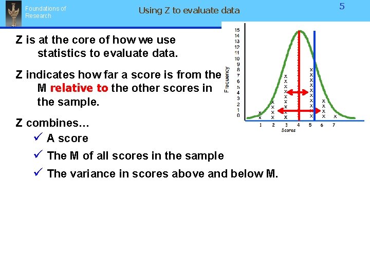
Foundations of Research Using Z to evaluate data Z is at the core of how we use statistics to evaluate data. Z indicates how far a score is from the M relative to the other scores in the sample. Z combines… ü A score ü The M of all scores in the sample ü The variance in scores above and below M. 5

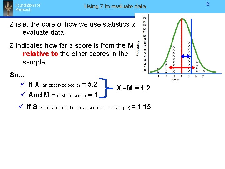
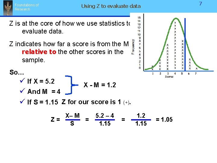
Foundations of Research Using Z to evaluate data Z is at the core of how we use statistics to evaluate data. Z indicates how far a score is from the M relative to the other scores in the sample. So… ü If X (an observed score) = 5. 2 ü And M (The Mean score) = 4 X - M = 1. 2 ü If S (Standard deviation of all scores in the sample) = 1. 15 6

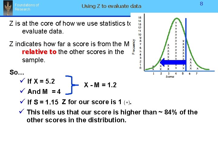
7 Using Z to evaluate data Foundations of Research Z is at the core of how we use statistics to evaluate data. Z indicates how far a score is from the M relative to the other scores in the sample. So… ü If X = 5. 2 X - M = 1. 2 ü And M = 4 ü If S = 1. 15 Z for our score is 1 (+). Z= X– M = S 5. 2 – 4 1. 15 = 1. 2 1. 15 = 1. 05

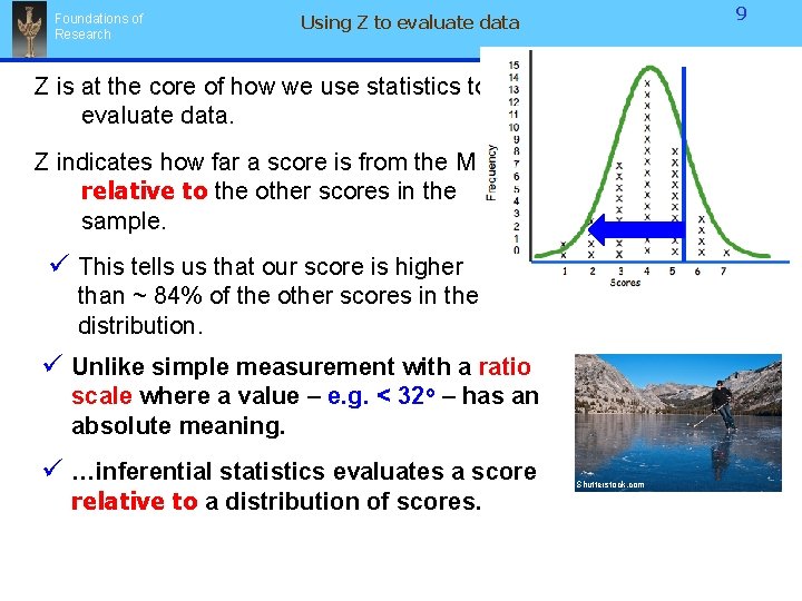
Foundations of Research Using Z to evaluate data Z is at the core of how we use statistics to evaluate data. Z indicates how far a score is from the M relative to the other scores in the sample. So… ü If X = 5. 2 X - M = 1. 2 ü And M = 4 ü If S = 1. 15 Z for our score is 1 (+). ü This tells us that our score is higher than ~ 84% of the other scores in the distribution. 8

Foundations of Research 9 Using Z to evaluate data Z is at the core of how we use statistics to evaluate data. Z indicates how far a score is from the M relative to the other scores in the sample. ü This tells us that our score is higher than ~ 84% of the other scores in the distribution. ü Unlike simple measurement with a ratio scale where a value – e. g. < 32 o – has an absolute meaning. ü …inferential statistics evaluates a score relative to a distribution of scores. Shutterstock. com

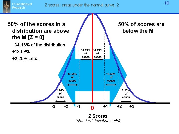
Foundations of Research 10 Z scores: areas under the normal curve, 2 50% of the scores in a distribution are above the M [Z = 0] 50% of scores are below the M 34. 13% of the distribution 34. 13% of of cases +13. 59% +2. 25%. . . etc. 13. 59% of cases 2. 25% of cases -3 -2 2. 25% of cases -1 0 0 +1 Z Scores +2 (standard deviation units) +3

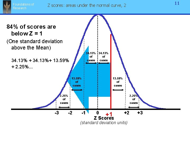
Foundations of Research 11 Z scores: areas under the normal curve, 2 84% of scores are below Z = 1 (One standard deviation above the Mean) 34. 13% of of cases 34. 13% + 34. 13%+ 13. 59% + 2. 25%. . . 13. 59% of cases 2. 25% of cases -3 -2 2. 25% of cases -1 0 +1 +1 Z Scores +2 (standard deviation units) +3

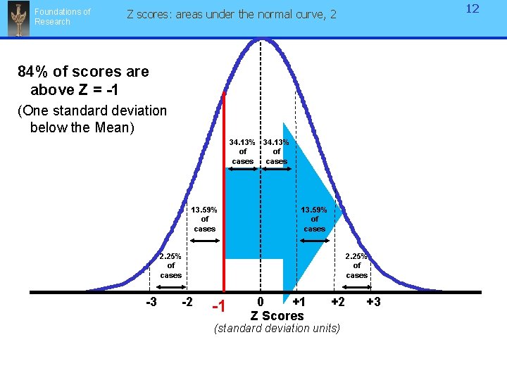
Foundations of Research 12 Z scores: areas under the normal curve, 2 84% of scores are above Z = -1 (One standard deviation below the Mean) 34. 13% of of cases 13. 59% of cases 2. 25% of cases -3 -2 2. 25% of cases -1 -1 0 +1 Z Scores +2 (standard deviation units) +3

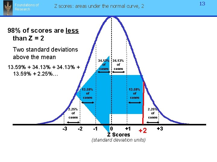
Foundations of Research 13 Z scores: areas under the normal curve, 2 98% of scores are less than Z = 2 Two standard deviations above the mean 34. 13% of of cases 13. 59% + 34. 13% + 13. 59% + 2. 25%… 13. 59% of cases 2. 25% of cases -3 -2 2. 25% of cases -1 0 +1 Z Scores +2 +2 (standard deviation units) +3

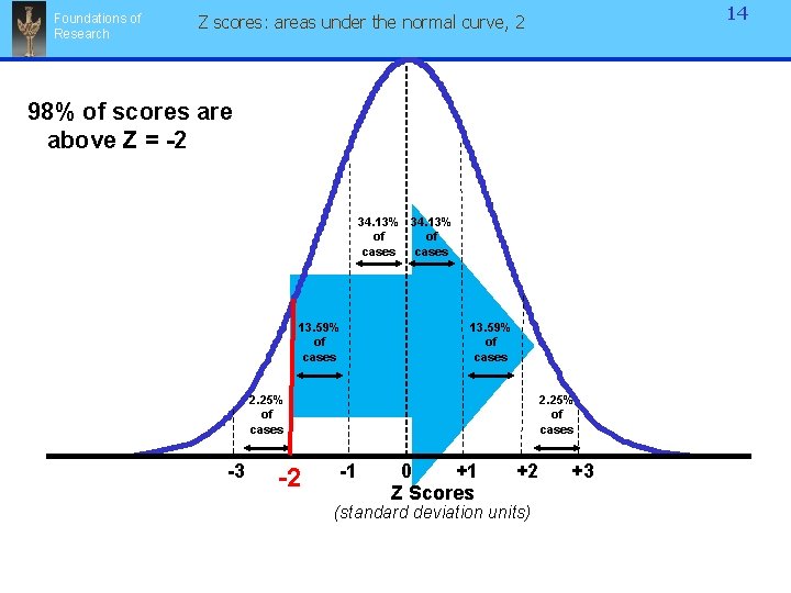
Foundations of Research 14 Z scores: areas under the normal curve, 2 98% of scores are above Z = -2 34. 13% of of cases 13. 59% of cases 2. 25% of cases -3 -2 -2 2. 25% of cases -1 0 +1 Z Scores +2 (standard deviation units) +3

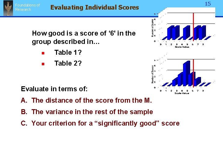
Foundations of Research Evaluating Individual Scores How good is a score of ‘ 6' in the group described in… n Table 1? n Table 2? Evaluate in terms of: A. The distance of the score from the M. B. The variance in the rest of the sample C. Your criterion for a “significantly good” score 15

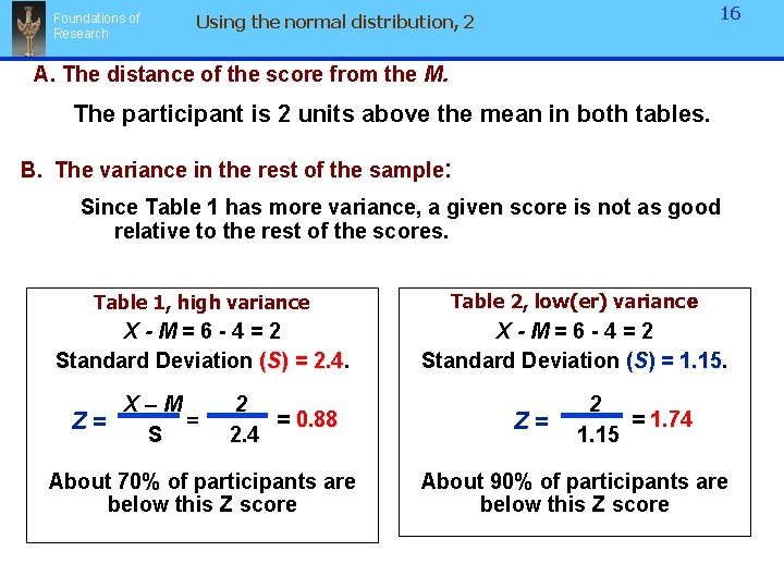
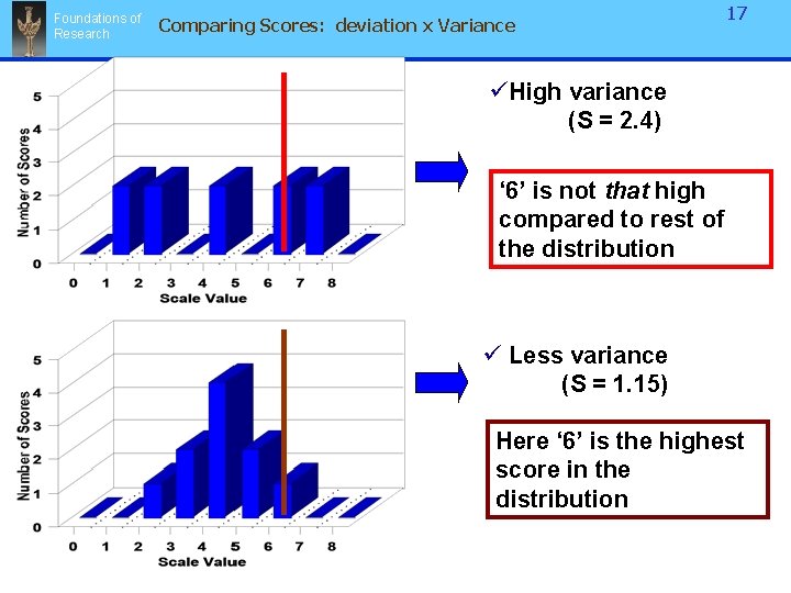
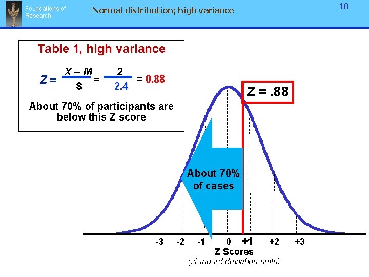
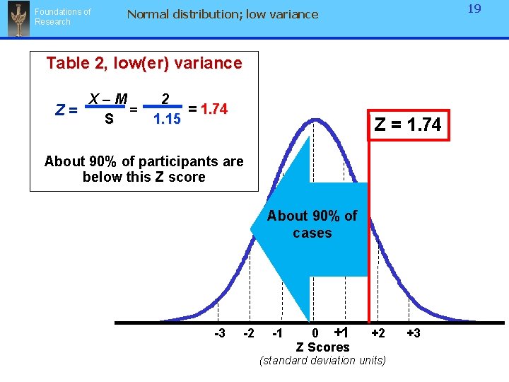
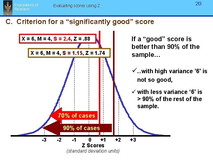
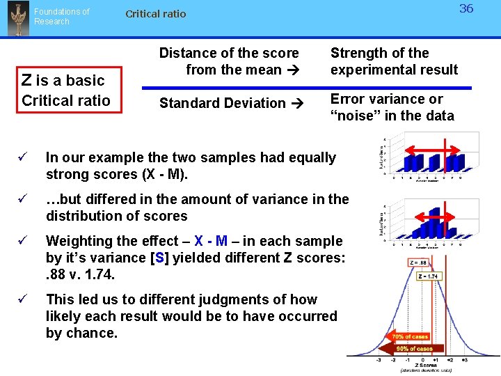
Foundations of Research 16 Using the normal distribution, 2 A. The distance of the score from the M. The participant is 2 units above the mean in both tables. B. The variance in the rest of the sample: Since Table 1 has more variance, a given score is not as good relative to the rest of the scores. Table 1, high variance Table 2, low(er) variance X-M=6 -4=2 Standard Deviation (S) = 2. 4 X-M=6 -4=2 Standard Deviation (S) = 1. 15 X–M = Z= S 2 = 0. 88 2. 4 About 70% of participants are below this Z score Z= 2 = 1. 74 1. 15 About 90% of participants are below this Z score

Foundations of Research Comparing Scores: deviation x Variance 17 üHigh variance (S = 2. 4) ‘ 6’ is not that high compared to rest of the distribution ü Less variance (S = 1. 15) Here ‘ 6’ is the highest score in the distribution

Foundations of Research 18 Normal distribution; high variance Table 1, high variance X–M = Z= S 2 = 0. 88 2. 4 Z =. 88 About 70% of participants are below this Z score About 70% of cases -3 -2 -1 0 +1 Z Scores +2 (standard deviation units) +3

Foundations of Research 19 Normal distribution; low variance Table 2, low(er) variance X–M = Z= S 2 = 1. 74 1. 15 Z = 1. 74 About 90% of participants are below this Z score About 90% of cases -3 -2 -1 0 +1 Z Scores +2 (standard deviation units) +3

20 Evaluating scores using Z Foundations of Research C. Criterion for a “significantly good” score If a “good” score is better than 90% of the sample… X = 6, M = 4, S = 2. 4, 2. 4 Z =. 88 X = 6, M = 4, S = 1. 15, 1. 15 Z = 1. 74 ü. . with high variance ’ 6' is not so good, ü with less variance ‘ 6’ is > 90% of the rest of the sample. 70% of cases 90% of cases -3 -2 -1 0 +1 Z Scores +2 (standard deviation units) +3

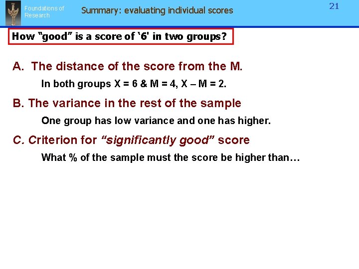
Foundations of Research Summary: evaluating individual scores How “good” is a score of ‘ 6' in two groups? A. The distance of the score from the M. In both groups X = 6 & M = 4, X – M = 2. B. The variance in the rest of the sample One group has low variance and one has higher. C. Criterion for “significantly good” score What % of the sample must the score be higher than… 21

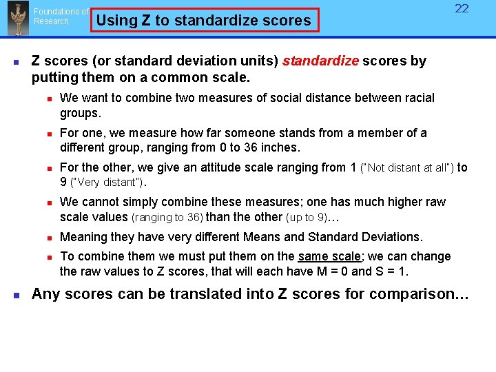
Foundations of Research n Z scores (or standard deviation units) standardize scores by putting them on a common scale. n n n n Using Z to standardize scores 22 We want to combine two measures of social distance between racial groups. For one, we measure how far someone stands from a member of a different group, ranging from 0 to 36 inches. For the other, we give an attitude scale ranging from 1 (“Not distant at all”) to 9 (“Very distant”). We cannot simply combine these measures; one has much higher raw scale values (ranging to 36) than the other (up to 9)… Meaning they have very different Means and Standard Deviations. To combine them we must put them on the same scale; we can change the raw values to Z scores, that will each have M = 0 and S = 1. Any scores can be translated into Z scores for comparison…

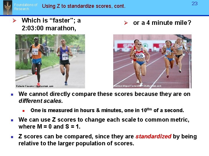
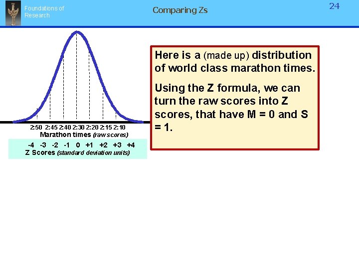
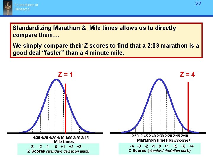
Foundations of Research Using Z to standardize scores, cont. Ø Which is “faster”; a 2: 03: 00 marathon, Roberto Caucino / Shutterstock. com n n Ø or a 4 minute mile? Gustavo Miguel Fernandes / Shutterstock. com We cannot directly compare these scores because they are on different scales. n n 23 One is measured in hours & minutes, one in 10 ths of a second. We can use Z scores to change each scale to common metric, where M = 0 and S = 1. Z scores can be compared, since they are standardized by being relative to the larger population of scores.

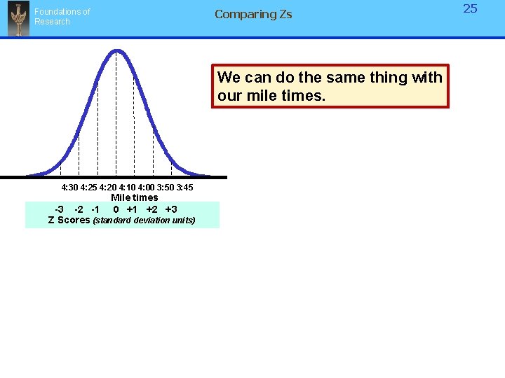
Foundations of Research Comparing Zs Here is a (made up) distribution of world class marathon times. 2: 50 2: 45 2: 40 2: 30 2: 20 2: 15 2: 10 Marathon times (raw scores) -4 -3 -2 -1 0 +1 +2 +3 +4 Z Scores (standard deviation units) Using the Z formula, we can turn the raw scores into Z scores, that have M = 0 and S = 1. 24

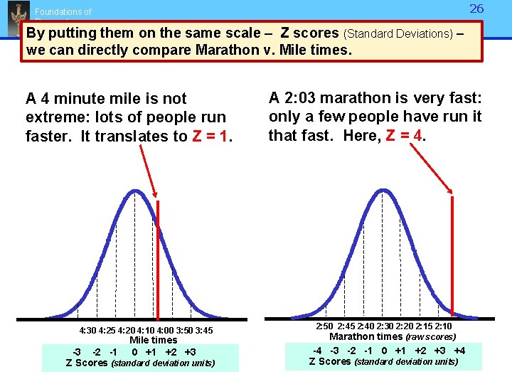
Comparing Zs Foundations of Research We can do the same thing with our mile times. 4: 30 4: 25 4: 20 4: 10 4: 00 3: 50 3: 45 Mile times 0 +1 +2 +3 -3 -2 -1 Z Scores (standard deviation units) 25

26 Foundations of Research By putting them on the same scale – Z scores (Standard Deviations) – we can directly compare Marathon v. Mile times. A 4 minute mile is not extreme: lots of people run faster. It translates to Z = 1. 4: 30 4: 25 4: 20 4: 10 4: 00 3: 50 3: 45 Mile times 0 +1 +2 +3 -3 -2 -1 Z Scores (standard deviation units) A 2: 03 marathon is very fast: only a few people have run it that fast. Here, Z = 4. 2: 50 2: 45 2: 40 2: 30 2: 20 2: 15 2: 10 Marathon times (raw scores) -4 -3 -2 -1 0 +1 +2 +3 +4 Z Scores (standard deviation units)

27 Foundations of Research Standardizing Marathon & Mile times allows us to directly compare them… We simply compare their Z scores to find that a 2: 03 marathon is a good deal “faster” than a 4 minute mile. Z=1 4: 30 4: 25 4: 20 4: 10 4: 00 3: 50 3: 45 Mile times 0 +1 +2 +3 -3 -2 -1 Z Scores (standard deviation units) Z=4 2: 50 2: 45 2: 40 2: 30 2: 20 2: 15 2: 10 Marathon times (raw scores) -4 -3 -2 -1 0 +1 +2 +3 +4 Z Scores (standard deviation units)

Foundations of Research 28 The critical ratio q Using Z scores to evaluate data q Testing hypotheses: the critical ratio. Click for nebular vs. catastrophic hypotheses about the origin of the solar system. (David Darling, Encyclopedia of Science. ) Illustration of the nebular hypothesis

Using statistics to test hypotheses: Foundations of Research 29 Core concept: ü No scientific finding is “absolutely” true. ü Any effect is probabilistic: Ø We use empirical data to infer how the world words Ø We evaluate inferences by how likely the effect would be to occur by chance. Ø We use the normal distribution to help us determine how likely an experimental outcome would be by chance alone.

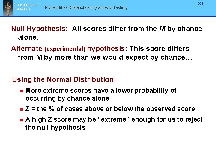
Foundations of Research Probabilities & Statistical Hypothesis Testing 30 Null Hypothesis: All scores differ from the M by chance alone. Scientific observations are “innocent until proven guilty”. If we compare two groups or test how far a score is from the mean, the odds of their being different by chance alone is always greater than 0. We cannot just take any result and call it meaningful, since any result may be due to chance, not the Independent Variable. So, we assume any result is by chance unless it is strong enough to be unlikely to occur randomly.

Foundations of Research Probabilities & Statistical Hypothesis Testing 31 Null Hypothesis: All scores differ from the M by chance alone. Alternate (experimental) hypothesis: This score differs from M by more than we would expect by chance… Using the Normal Distribution: n n n More extreme scores have a lower probability of occurring by chance alone Z = the % of cases above or below the observed score A high Z score may be “extreme” enough for us to reject the null hypothesis

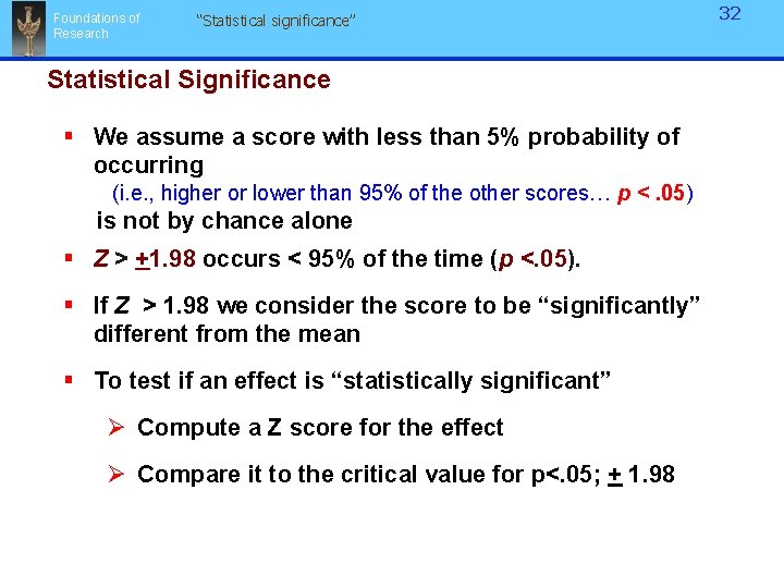
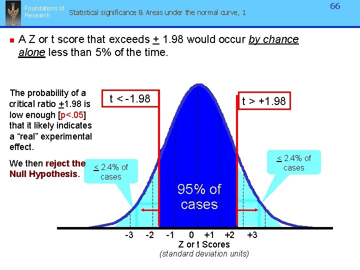
Foundations of Research “Statistical significance” Statistical Significance § We assume a score with less than 5% probability of occurring (i. e. , higher or lower than 95% of the other scores… p <. 05) is not by chance alone § Z > +1. 98 occurs < 95% of the time (p <. 05). § If Z > 1. 98 we consider the score to be “significantly” different from the mean § To test if an effect is “statistically significant” Ø Compute a Z score for the effect Ø Compare it to the critical value for p<. 05; + 1. 98 32

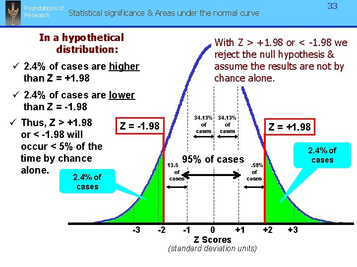
Foundations of Research 33 Statistical significance & Areas under the normal curve In a hypothetical distribution: With Z > +1. 98 or < -1. 98 we reject the null hypothesis & assume the results are not by chance alone. ü 2. 4% of cases are higher than Z = +1. 98 ü 2. 4% of cases are lower than Z = -1. 98 ü Thus, Z > +1. 98 or < -1. 98 will occur < 5% of the time by chance alone. 34. 13% of of cases Z = -1. 98 Z = +1. 98 2. 4% of cases 95% of cases 13. 59% of cases 2. 4% of cases 2. 25% of cases -3 -2 2. 25% of cases -1 0 +1 Z Scores (standard deviation units) +2 +3

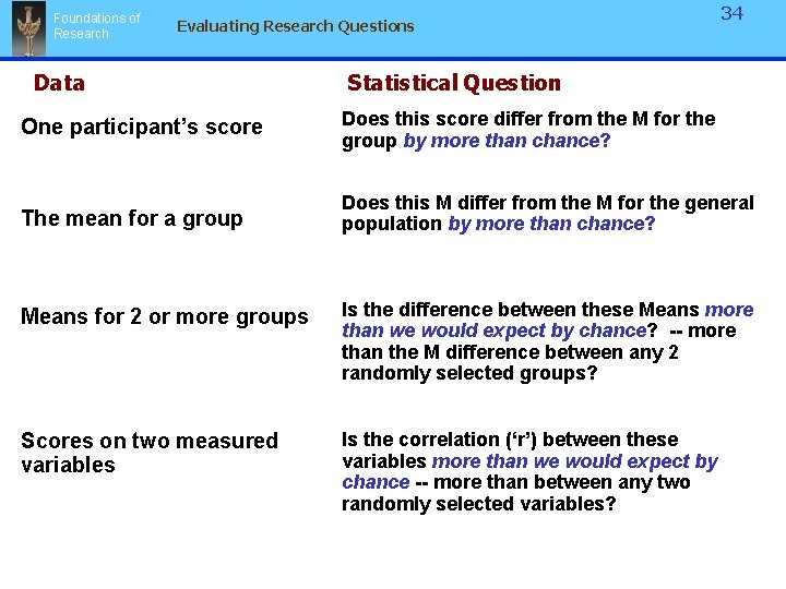
Foundations of Research Evaluating Research Questions Data 34 Statistical Question One participant’s score Does this score differ from the M for the group by more than chance? The mean for a group Does this M differ from the M for the general population by more than chance? Means for 2 or more groups Is the difference between these Means more than we would expect by chance? -- more than the M difference between any 2 randomly selected groups? Scores on two measured variables Is the correlation (‘r’) between these variables more than we would expect by chance -- more than between any two randomly selected variables?

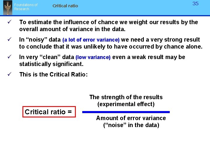
Foundations of Research 35 Critical ratio ü To estimate the influence of chance we weight our results by the overall amount of variance in the data. ü In “noisy” data (a lot of error variance) we need a very strong result to conclude that it was unlikely to have occurred by chance alone. ü In very “clean” data (low variance) even a weak result may be statistically significant. ü This is the Critical Ratio: The strength of the results (experimental effect) Critical ratio = Amount of error variance (“noise” in the data)

Foundations of Research Z is a basic Critical ratio 36 Critical ratio Distance of the score from the mean Strength of the experimental result Standard Deviation Error variance or “noise” in the data ü In our example the two samples had equally strong scores (X - M). ü …but differed in the amount of variance in the distribution of scores ü Weighting the effect – X - M – in each sample by it’s variance [S] yielded different Z scores: . 88 v. 1. 74. ü This led us to different judgments of how likely each result would be to have occurred by chance.

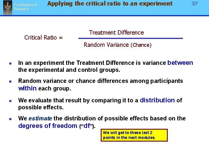
Foundations of Research Applying the critical ratio to an experiment Critical Ratio = 37 Treatment Difference Random Variance (Chance) n n In an experiment the Treatment Difference is variance between the experimental and control groups. Random variance or chance differences among participants within each group. We evaluate that result by comparing it to a distribution of possible effects. We estimate the distribution of possible effects based on the degrees of freedom (“df”). We will get to these last 2 points in the next modules.

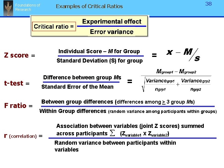
Individual Score – M for Group Z score = t-test = F ratio = 38 Examples of Critical Ratios Foundations of Research Standard Deviation (S) for group Difference between group Ms Standard Error of the Mean = = Between group differences (differences among > 3 group Ms) Within Group differences (random variance among participants within groups) r (correlation) = Association between variables (joint Z scores) summed across participants (Zvariable 1 x Zvariable 2) Random variance between participants within variables

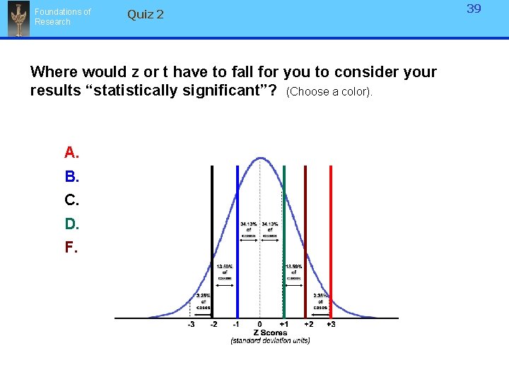
Foundations of Research Quiz 2 Where would z or t have to fall for you to consider your results “statistically significant”? (Choose a color). A. B. C. D. F. 39

Foundations of Research 40 Quiz 2 Where would z or t have to fall for you to consider your results “statistically significant”? (Choose a color). ü Both of these are correct. A. B. C. D. F. ü A Z or t score greater than or less than 1. 98 is consided it significant. ü This means that the result would occur < 5% of the time by chance alone (p < 05).

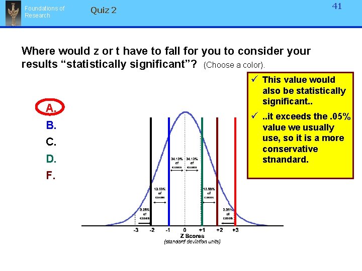
Foundations of Research 41 Quiz 2 Where would z or t have to fall for you to consider your results “statistically significant”? (Choose a color). ü This value would A. B. C. D. F. also be statistically significant. . ü. . it exceeds the. 05% value we usually use, so it is a more conservative stnandard.

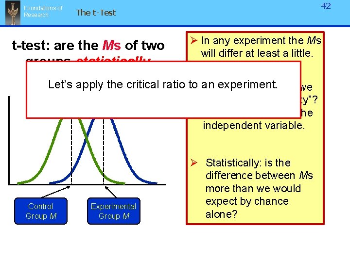
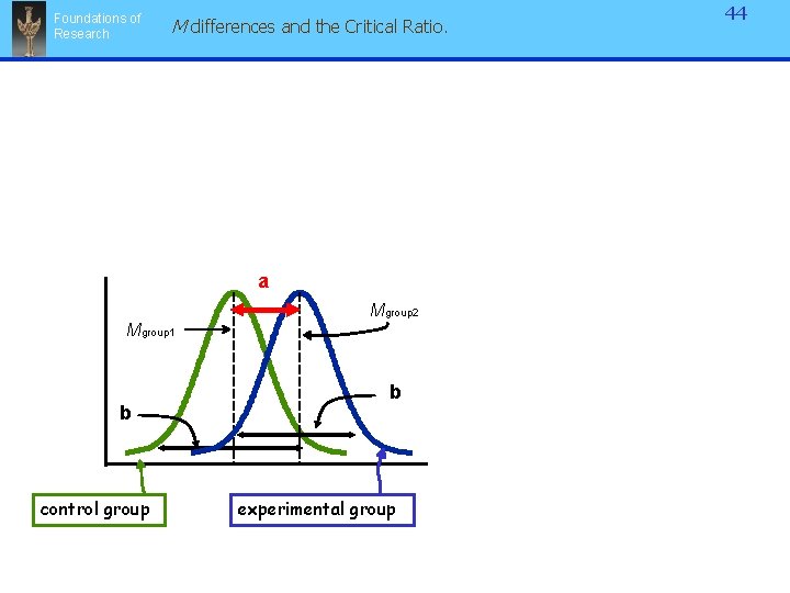
Foundations of Research 42 The t-Test Ø In any experiment the Ms t-test: are the Ms of two will differ at least a little. groups statistically different from Let’s apply theeach critical ratio to experiment. Ø an Does the difference we other? observe reflect “reality”? … i. e. , really due to the independent variable. Control Group M Experimental Group M Ø Statistically: is the difference between Ms more than we would expect by chance alone?

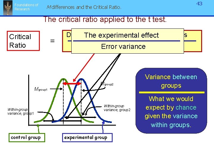
Foundations of Research 43 M differences and the Critical Ratio. The critical ratio applied to the t test. Critical Ratio = Difference Ms foreffect the two groups The between experimental Variability groups (error) Errorwithin variance Mgroup 2 Mgroup 1 Within-group variance, group 1 control group Within-group variance, group 2 experimental group Variance between groups What we would expect by chance given the variance within groups.

Foundations of Research M differences and the Critical Ratio. a Mgroup 2 Mgroup 1 b control group b experimental group 44

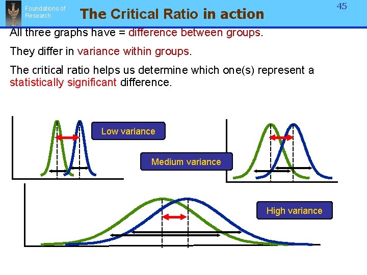
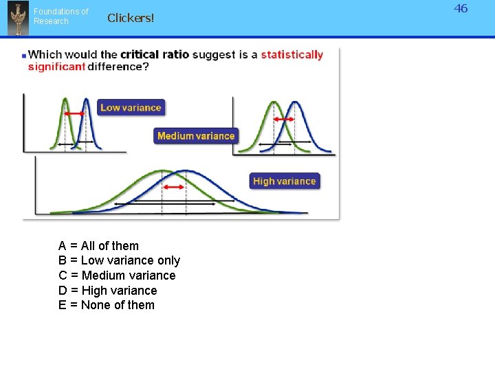
Foundations of Research 45 The Critical Ratio in action All three graphs have = difference between groups. They differ in variance within groups. The critical ratio helps us determine which one(s) represent a statistically significant difference. Low variance Medium variance High variance

Foundations of Research Clickers! A = All of them B = Low variance only C = Medium variance D = High variance E = None of them 46

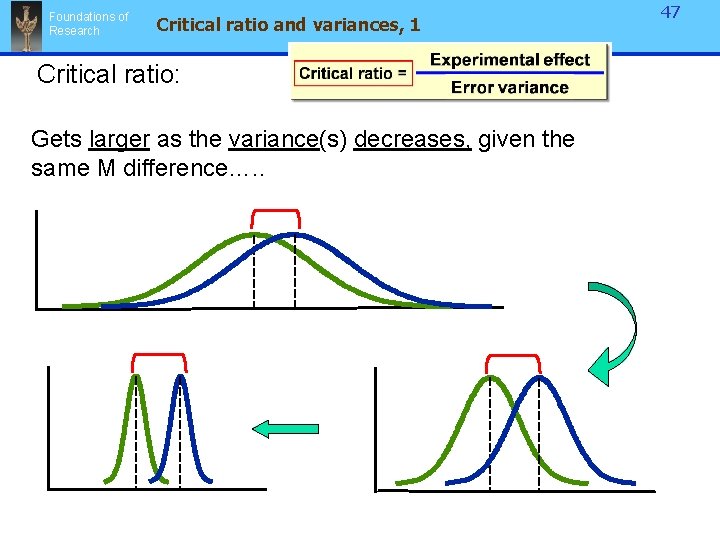
Foundations of Research Critical ratio and variances, 1 Critical ratio: Gets larger as the variance(s) decreases, given the same M difference…. . 47

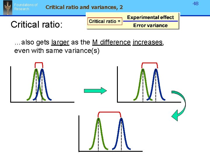
Foundations of Research Critical ratio and variances, 2 Critical ratio: …also gets larger as the M difference increases, even with same variance(s) 48

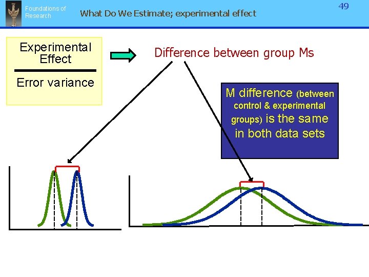
Foundations of Research What Do We Estimate; experimental effect Experimental Effect Error variance Difference between group Ms M difference (between control & experimental is the same in both data sets groups) 49

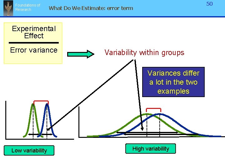
Foundations of Research 50 What Do We Estimate: error term Experimental Effect Error variance Variability within groups Variances differ a lot in the two examples Low variability High variability

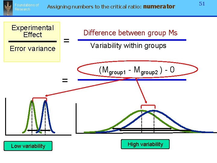
Foundations of Research Assigning numbers to the critical ratio: Experimental Effect Error variance = = Low variability numerator Difference between group Ms Variability within groups (Mgroup 1 - Mgroup 2 ) - 0 High variability 51

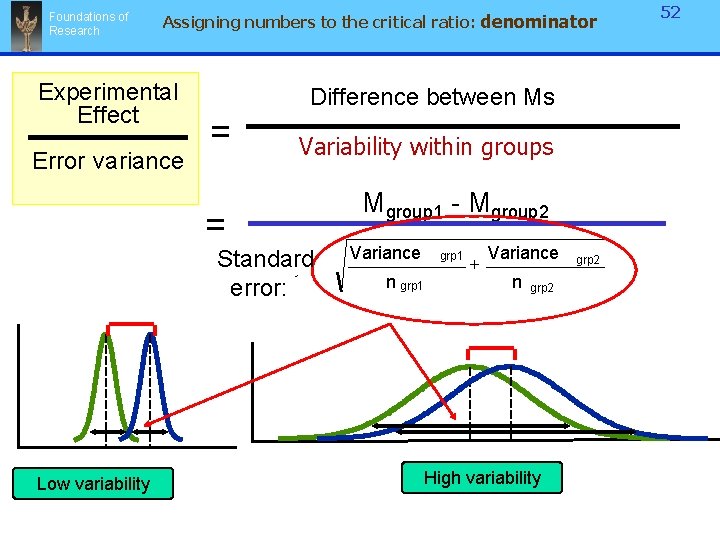
Foundations of Research Assigning numbers to the critical ratio: denominator Experimental Effect Error variance Difference between Ms = Variability within groups = Standard error: Low variability Mgroup 1 - Mgroup 2 Variance grp 1 n grp 1 + Variance n grp 2 High variability grp 2 52

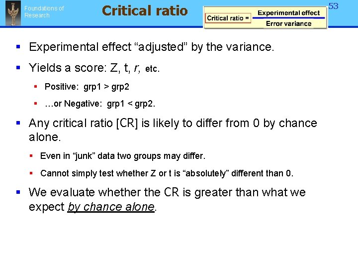
Foundations of Research Critical ratio § Experimental effect “adjusted” by the variance. § Yields a score: Z, t, r, etc. § Positive: grp 1 > grp 2 § …or Negative: grp 1 < grp 2. § Any critical ratio [CR] is likely to differ from 0 by chance alone. § Even in “junk” data two groups may differ. § Cannot simply test whether Z or t is “absolutely” different than 0. § We evaluate whether the CR is greater than what we expect by chance alone. 53

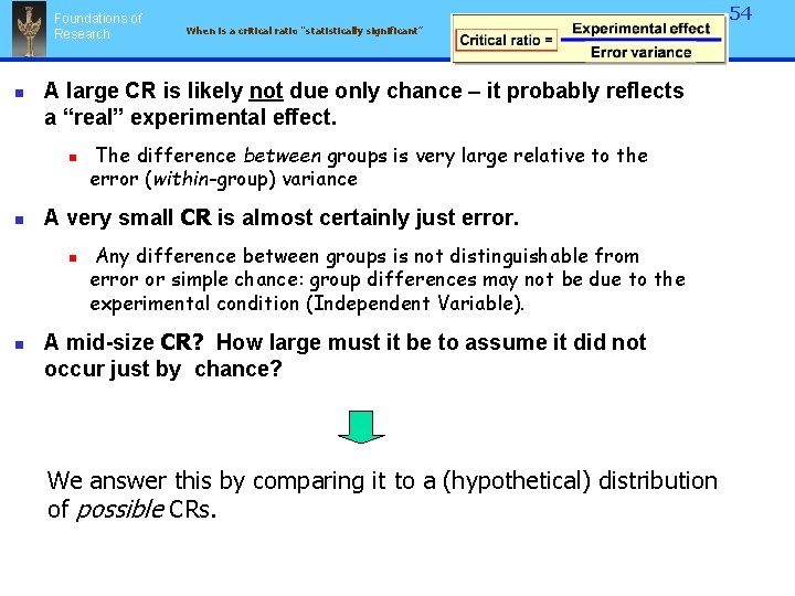
Foundations of Research n A large CR is likely not due only chance – it probably reflects a “real” experimental effect. n n The difference between groups is very large relative to the error (within-group) variance A very small CR is almost certainly just error. n n 54 When is a critical ratio “statistically significant” Any difference between groups is not distinguishable from error or simple chance: group differences may not be due to the experimental condition (Independent Variable). A mid-size CR? How large must it be to assume it did not occur just by chance? We answer this by comparing it to a (hypothetical) distribution of possible CRs.

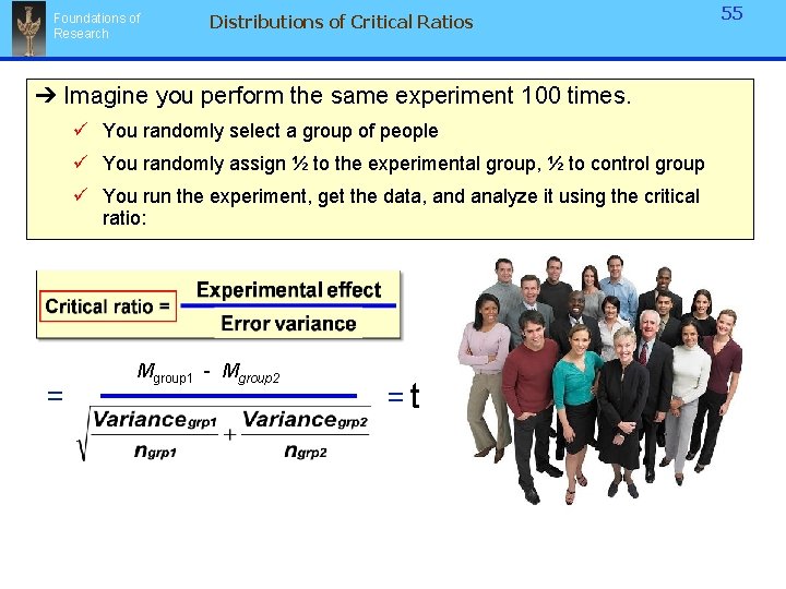
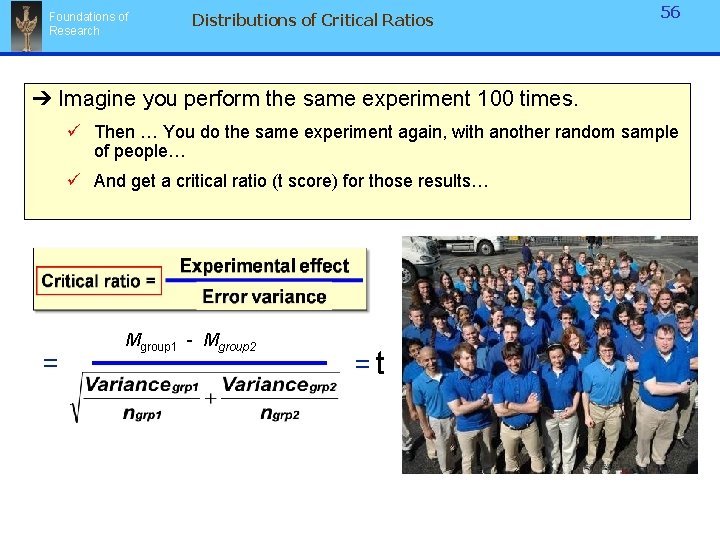
Foundations of Research Distributions of Critical Ratios ➔ Imagine you perform the same experiment 100 times. ü You randomly select a group of people ü You randomly assign ½ to the experimental group, ½ to control group ü You run the experiment, get the data, and analyze it using the critical ratio: = Mgroup 1 - Mgroup 2 =t 55

Foundations of Research Distributions of Critical Ratios 56 ➔ Imagine you perform the same experiment 100 times. ü Then … You do the same experiment again, with another random sample of people… ü And get a critical ratio (t score) for those results… = Mgroup 1 - Mgroup 2 =t

Foundations of Research Distributions of Critical Ratios ➔ Imagine you perform the same experiment 100 times. ü And you get yet another sample… ü And get a critical ratio (t score) for those results… = Mgroup 1 - Mgroup 2 =t 57

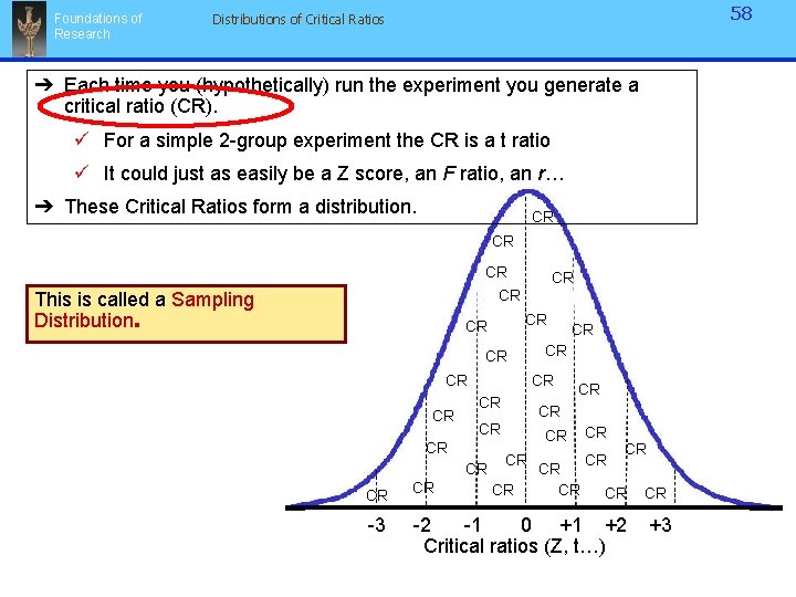
Foundations of Research 58 Distributions of Critical Ratios ➔ Each time you (hypothetically) run the experiment you generate a critical ratio (CR). ü For a simple 2 -group experiment the CR is a t ratio ü It could just as easily be a Z score, an F ratio, an r… ➔ These Critical Ratios form a distribution. CR CR CR This is called a Sampling Distribution. CR CR CR -3 CR CR CR CR CR -2 -1 0 +1 +2 Critical ratios (Z, t…) +3

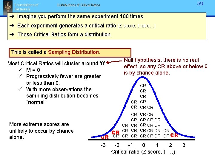
Foundations of Research 59 Distributions of Critical Ratios ➔ Imagine you perform the same experiment 100 times. ➔ Each experiment generates a critical ratio [Z score, t ratio…] ➔ These Critical Ratios form a distribution This is called a Sampling Distribution. Most Critical Ratios will cluster around ‘ 0’ ü M=0 ü Progressively fewer are greater or less than 0. ü With more observations the sampling distribution becomes “normal” More extreme scores are unlikely to occur by chance alone. CR -3 Null hypothesis; there is no real effect, so any CR above or below 0 is by chance alone. CR CR CR CR CR CR CR CR CR -2 -1 0 1 2 Critical ratio (Z score, t, …) 3

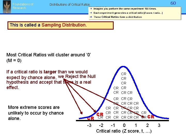
Foundations of Research 60 Distributions of Critical Ratios This is called a Sampling Distribution. Most Critical Ratios will cluster around ‘ 0’ (M = 0) If a critical ratio is larger than we would expect by chance alone, we Reject the Null hypothesis and accept that there is a real effect. More extreme scores are unlikely to occur by chance alone. CR -3 CR CR CR CR CR CR CR CR CR -2 -1 0 1 2 Critical ratio (Z score, t, …) 3

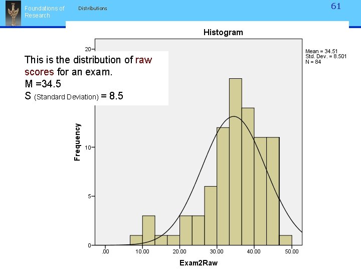
Foundations of Research 61 Distributions This is the distribution of raw scores for an exam. M =34. 5 S (Standard Deviation) = 8. 5 Statistics Introduction 2.

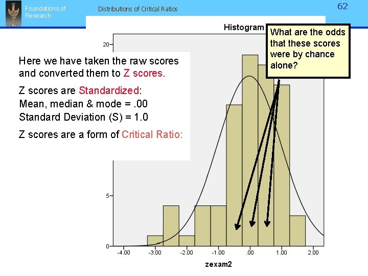
Foundations of Research Distributions of Critical Ratios Here we have taken the raw scores and converted them to Z scores are Standardized: Mean, median & mode =. 00 Standard Deviation (S) = 1. 0 Z scores are a form of Critical Ratio: Statistics Introduction 2. 62 What are the odds that these scores were by chance alone?

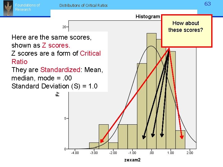
Foundations of Research 63 Distributions of Critical Ratios How about these scores? Here are the same scores, shown as Z scores are a form of Critical Ratio They are Standardized: Mean, median, mode =. 00 Standard Deviation (S) = 1. 0

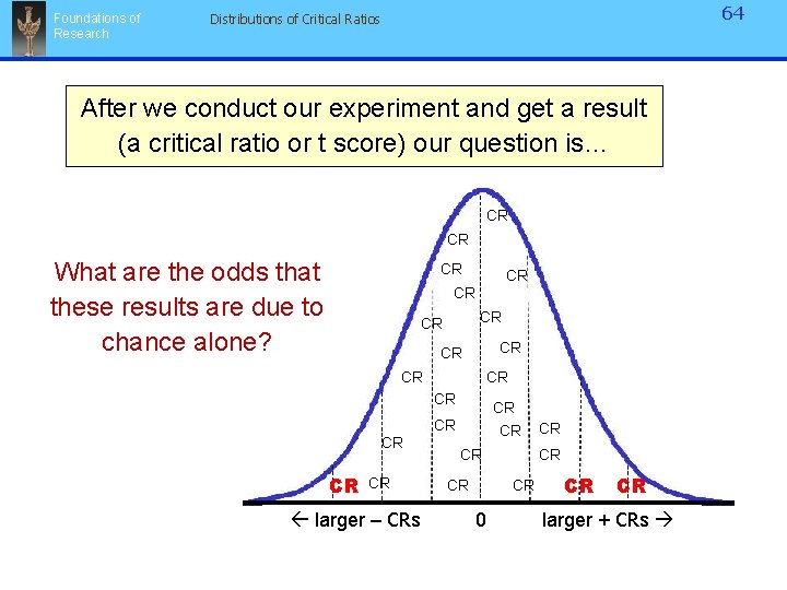
Foundations of Research 64 Distributions of Critical Ratios After we conduct our experiment and get a result (a critical ratio or t score) our question is… CR CR What are the odds that these results are due to chance alone? CR CR CR CR larger – CRs CR CR CR 0 CR CR CR larger + CRs

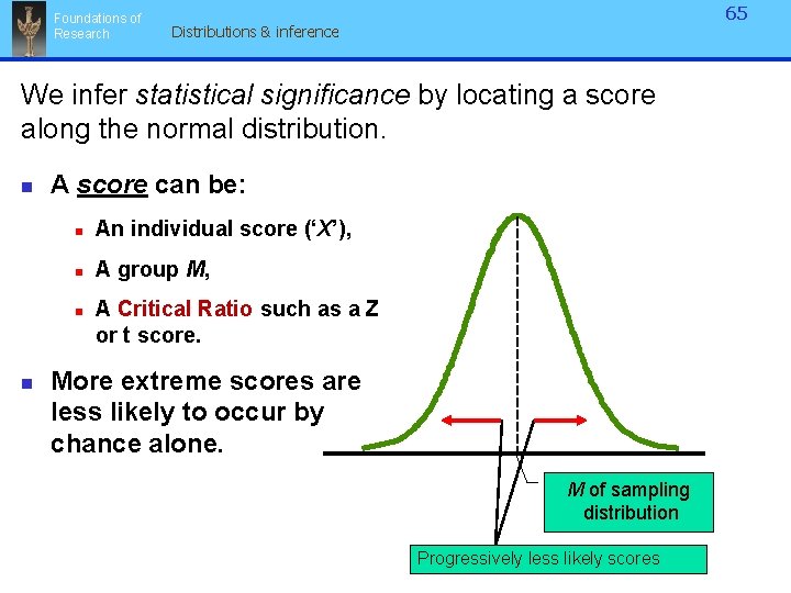
Foundations of Research 65 Distributions & inference We infer statistical significance by locating a score along the normal distribution. n A score can be: n An individual score (‘X’), n A group M, n n A Critical Ratio such as a Z or t score. More extreme scores are less likely to occur by chance alone. M of sampling distribution Progressively less likely scores

66 Foundations of Statistical significance & Areas under the normal curve, 1 Research n A Z or t score that exceeds + 1. 98 would occur by chance alone less than 5% of the time. The probability of a critical ratio +1. 98 is low enough [p<. 05] that it likely indicates a “real” experimental effect. t < -1. 98 t > +1. 98 < 2. 4% of cases We then reject the < 2. 4% of Null Hypothesis. cases 95% of cases -3 -2 -1 0 +1 +2 Z or t Scores +3 (standard deviation units)

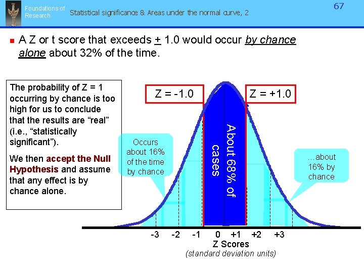
67 Foundations of Statistical significance & Areas under the normal curve, 2 Research n A Z or t score that exceeds + 1. 0 would occur by chance alone about 32% of the time. We then accept the Null Hypothesis and assume that any effect is by chance alone. Z = -1. 0 Occurs about 16% of the time by chance -3 Z = +1. 0 About 68% of cases The probability of Z = 1 occurring by chance is too high for us to conclude that the results are “real” (i. e. , “statistically significant”). -2 -1 0 +1 +2 Z Scores …about 16% by chance +3 (standard deviation units)

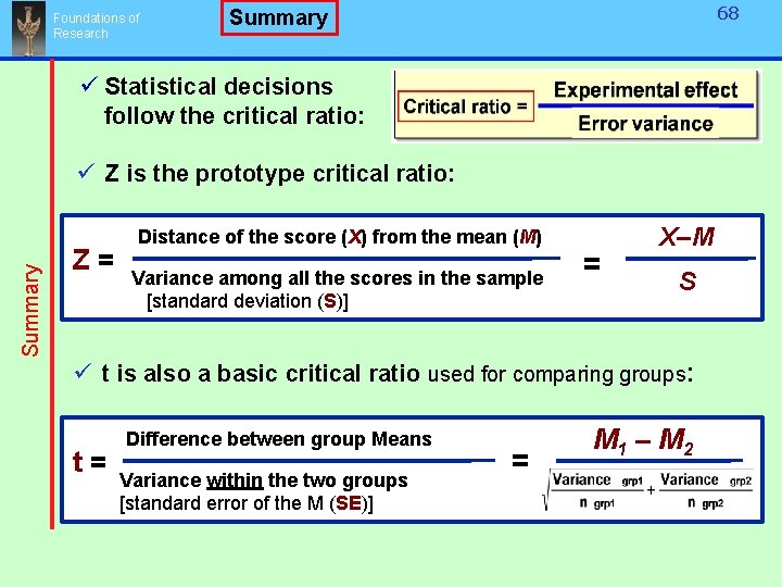
Foundations of Research 68 Summary ü Statistical decisions follow the critical ratio: Summary ü Z is the prototype critical ratio: Z= Distance of the score (X) from the mean (M) Variance among all the scores in the sample [standard deviation (S)] = X–M S ü t is also a basic critical ratio used for comparing groups: t= Difference between group Means Variance within the two groups [standard error of the M (SE)] = M 1 – M 2

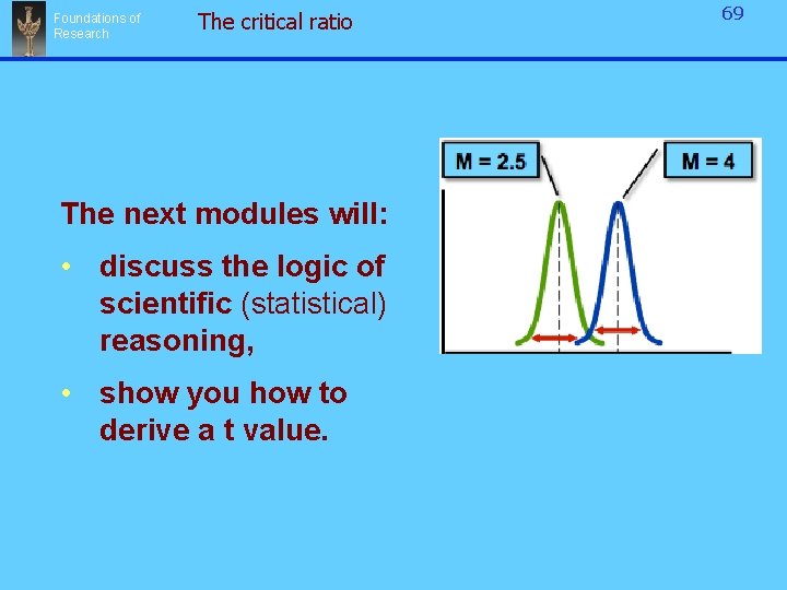
Foundations of Research The critical ratio The next modules will: • discuss the logic of scientific (statistical) reasoning, • show you how to derive a t value. 69