Foundations of Programming Languages Introduction to Lambda Calculus

Foundations of Programming Languages: Introduction to Lambda Calculus Adapted from Lectures by Profs Aiken and Necula of Univ. of California at Berkeley CS 776 Prasad 1

Lecture Outline • Why study lambda calculus? • Lambda calculus – Syntax – Evaluation – Relationship to programming languages • Next time: type systems for lambda calculus CS 776 Prasad 2

Lambda Calculus. History. • A framework developed in 1930 s by Alonzo Church to study computations with functions • Church wanted a minimal notation – to expose only what is essential • Two operations with functions are essential: – function creation – function application CS 776 Prasad 3

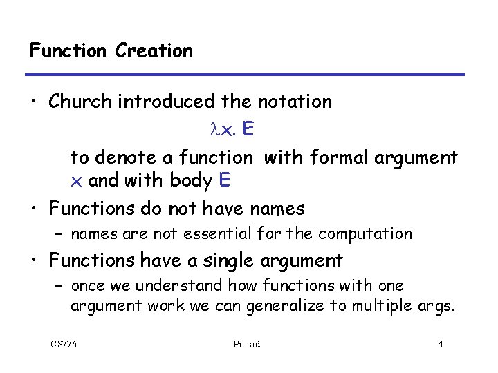
Function Creation • Church introduced the notation lx. E to denote a function with formal argument x and with body E • Functions do not have names – names are not essential for the computation • Functions have a single argument – once we understand how functions with one argument work we can generalize to multiple args. CS 776 Prasad 4

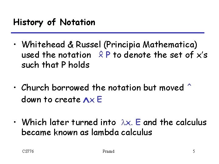
History of Notation • Whitehead & Russel (Principia Mathematica) x P to denote the set of x’s used the notation ˆ such that P holds • Church borrowed the notation but moved ˆ down to create Ùx E • Which later turned into lx. E and the calculus became known as lambda calculus CS 776 Prasad 5

Function Application • The only thing that we can do with a function is to apply it to an argument • Church used the notation E 1 E 2 to denote the application of function E 1 to actual argument E 2 • All functions are applied to a single argument CS 776 Prasad 6

Why Study Lambda Calculus? • l-calculus had a tremendous influence on the design and analysis of programming languages • Realistic languages are too large and complex to study from scratch as a whole • Typical approach is to modularize the study into one feature at a time – E. g. , recursion, looping, exceptions, objects, etc. • Then we assemble the features together CS 776 Prasad 7

Why Study Lambda Calculus? • l-calculus is the standard testbed for studying programming language features – Because of its minimality – Despite its syntactic simplicity the l-calculus can easily encode: • numbers, recursive data types, modules, imperative features, exceptions, etc. • Certain language features necessitate more substantial extensions to l-calculus: – for distributed & parallel languages: p-calculus – for object oriented languages: -calculus CS 776 Prasad 8

Why Study Lambda Calculus? “Whatever the next 700 languages turn out to be, they will surely be variants of lambda calculus. ” (Landin 1966) CS 776 Prasad 9

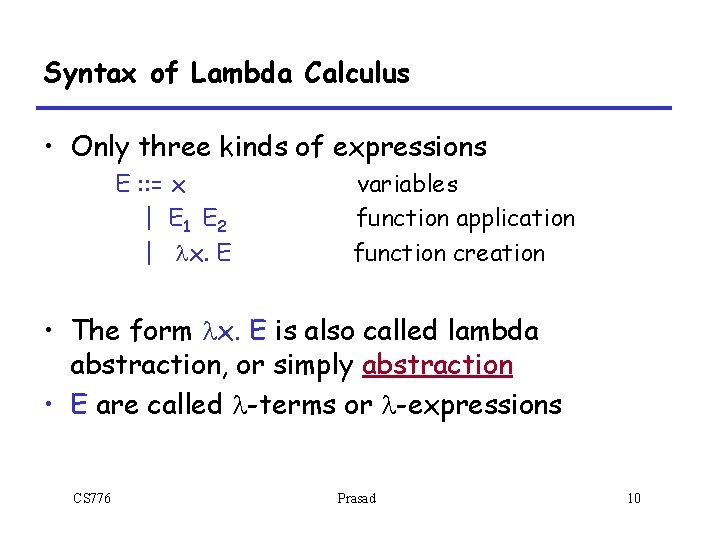
Syntax of Lambda Calculus • Only three kinds of expressions E : : = x | E 1 E 2 | lx. E variables function application function creation • The form lx. E is also called lambda abstraction, or simply abstraction • E are called l-terms or l-expressions CS 776 Prasad 10

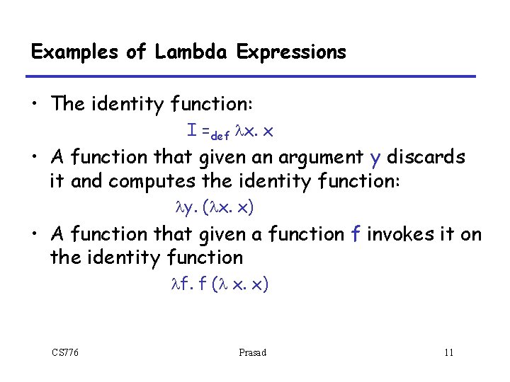
Examples of Lambda Expressions • The identity function: I =def lx. x • A function that given an argument y discards it and computes the identity function: ly. (lx. x) • A function that given a function f invokes it on the identity function lf. f (l x. x) CS 776 Prasad 11

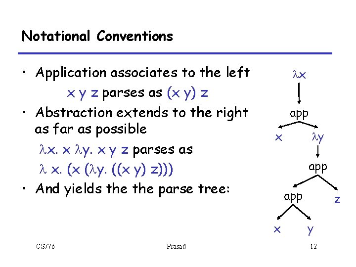
Notational Conventions • Application associates to the left x y z parses as (x y) z • Abstraction extends to the right as far as possible lx. x ly. x y z parses as l x. (x (ly. ((x y) z))) • And yields the parse tree: lx app app x CS 776 Prasad ly z y 12

Scope of Variables • As in all languages with variables, it is important to discuss the notion of scope – Recall: the scope of an identifier is the portion of a program where the identifier is accessible • An abstraction lx. E binds variable x in E – – x is the newly introduced variable E is the scope of x we say x is bound in lx. E Just like formal function arguments are bound in the function body CS 776 Prasad 13

Free and Bound Variables • A variable is said to be free in E if it is not bound in E • We can define the free variables of an expression E recursively as follows: Free(x) = { x} Free(E 1 E 2) = Free(E 1) È Free(E 2) Free(lx. E) = Free(E) - { x } • Example: Free(lx. x (ly. x y z)) = { z } • Free variables are declared outside the term CS 776 Prasad 14

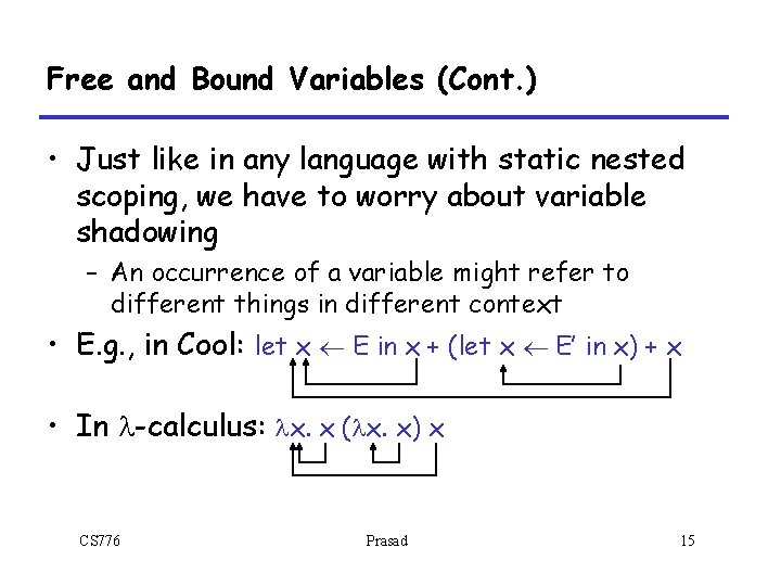
Free and Bound Variables (Cont. ) • Just like in any language with static nested scoping, we have to worry about variable shadowing – An occurrence of a variable might refer to different things in different context • E. g. , in Cool: let x ¬ E in x + (let x ¬ E’ in x) + x • In l-calculus: lx. x (lx. x) x CS 776 Prasad 15

Renaming Bound Variables • Two l-terms that can be obtained from each other by a renaming of the bound variables are considered identical • Example: lx. x is identical to ly. y and to lz. z • Intuition: – by changing the name of a formal argument and of all its occurrences in the function body, the behavior of the function does not change – in l-calculus such functions are considered identical CS 776 Prasad 16

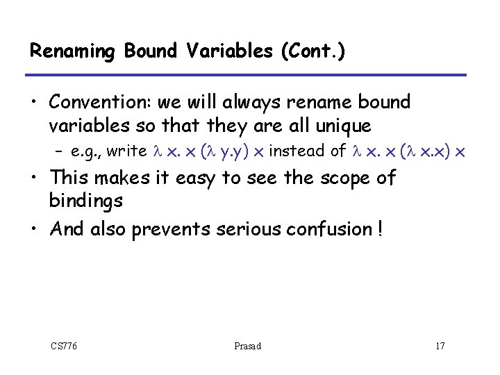
Renaming Bound Variables (Cont. ) • Convention: we will always rename bound variables so that they are all unique – e. g. , write l x. x (l y. y) x instead of l x. x (l x. x) x • This makes it easy to see the scope of bindings • And also prevents serious confusion ! CS 776 Prasad 17

Substitution • The substitution of E’ for x in E (written [E’/x]E ) – Step 1. Rename bound variables in E and E’ so they are unique – Step 2. Perform the textual substitution of E’ for x in E • Example: [y (lx. x) / x] ly. (lx. x) y x – After renaming: [y (lv. v)/x] lz. (lu. u) z x – After substitution: lz. (lu. u) z (y (lv. v)) CS 776 Prasad 18

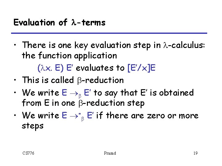
Evaluation of l-terms • There is one key evaluation step in l-calculus: the function application (lx. E) E’ evaluates to [E’/x]E • This is called b-reduction • We write E ®b E’ to say that E’ is obtained from E in one b-reduction step • We write E ®*b E’ if there are zero or more steps CS 776 Prasad 19

Examples of Evaluation • The identity function: (lx. x) E ® [E / x] x = E • Another example with the identity: (lf. f (lx. x)) (lx. x) ® [lx. x / f] f (lx. x)) = [(lx. x) / f] f (ly. y)) = (lx. x) (ly. y) ® [ly. y /x] x = ly. y • A non-terminating evaluation: (lx. xx) ® [lx. xx / x]xx = [ly. yy / x] xx = (ly. yy) ® … CS 776 Prasad 20

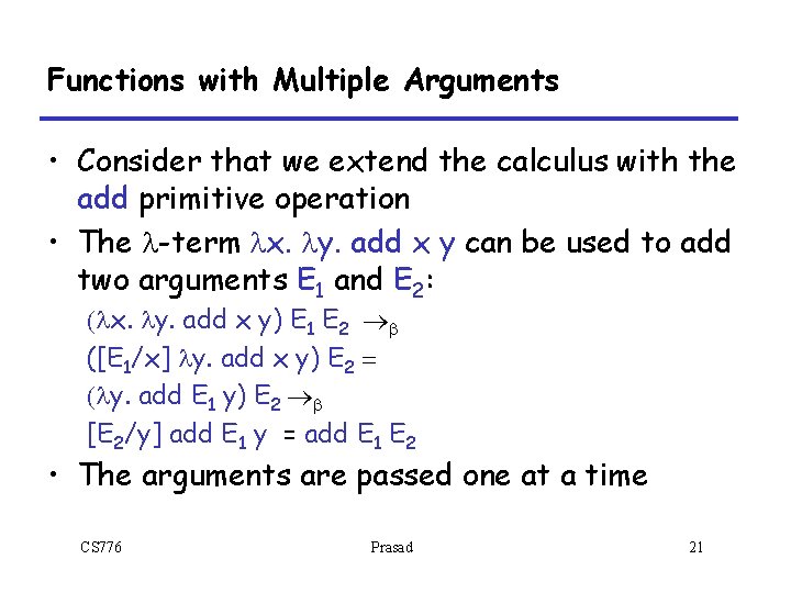
Functions with Multiple Arguments • Consider that we extend the calculus with the add primitive operation • The l-term lx. ly. add x y can be used to add two arguments E 1 and E 2: (lx. ly. add x y) E 1 E 2 ®b ([E 1/x] ly. add x y) E 2 = (ly. add E 1 y) E 2 ®b [E 2/y] add E 1 y = add E 1 E 2 • The arguments are passed one at a time CS 776 Prasad 21

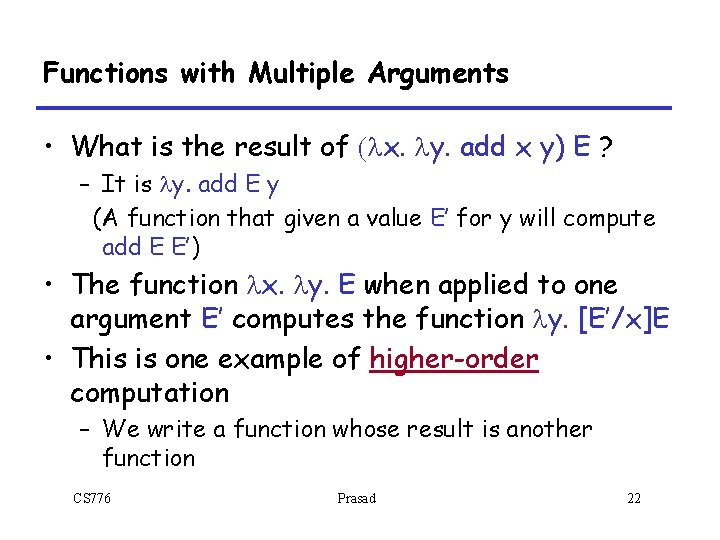
Functions with Multiple Arguments • What is the result of (lx. ly. add x y) E ? – It is ly. add E y (A function that given a value E’ for y will compute add E E’) • The function lx. ly. E when applied to one argument E’ computes the function ly. [E’/x]E • This is one example of higher-order computation – We write a function whose result is another function CS 776 Prasad 22

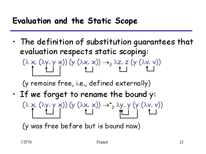
Evaluation and the Static Scope • The definition of substitution guarantees that evaluation respects static scoping: (l x. (ly. y x)) (y (lx. x)) ®b lz. z (y (lv. v)) (y remains free, i. e. , defined externally) • If we forget to rename the bound y: (l x. (ly. y x)) (y (lx. x)) ®*b ly. y (y (lv. v)) (y was free before but is bound now) CS 776 Prasad 23

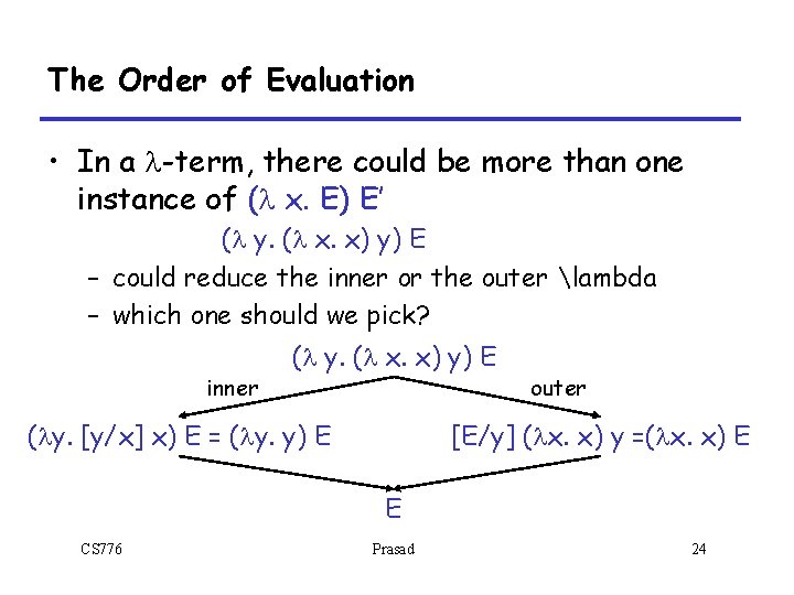
The Order of Evaluation • In a l-term, there could be more than one instance of (l x. E) E’ (l y. (l x. x) y) E – could reduce the inner or the outer lambda – which one should we pick? inner (l y. (l x. x) y) E (ly. [y/x] x) E = (ly. y) E outer [E/y] (lx. x) y =(lx. x) E E CS 776 Prasad 24

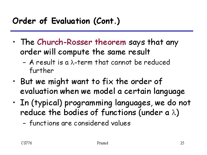
Order of Evaluation (Cont. ) • The Church-Rosser theorem says that any order will compute the same result – A result is a l-term that cannot be reduced further • But we might want to fix the order of evaluation when we model a certain language • In (typical) programming languages, we do not reduce the bodies of functions (under a l) – functions are considered values CS 776 Prasad 25

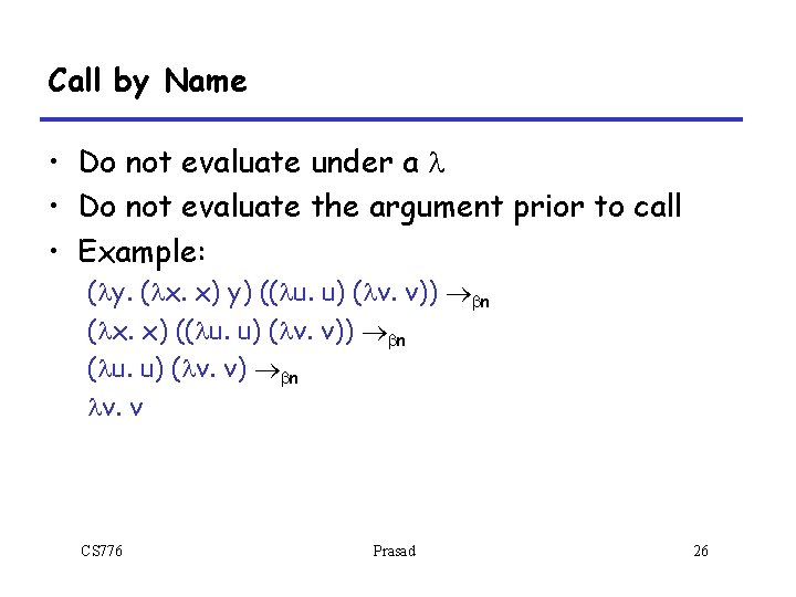
Call by Name • Do not evaluate under a l • Do not evaluate the argument prior to call • Example: (ly. (lx. x) y) ((lu. u) (lv. v)) ®bn (lx. x) ((lu. u) (lv. v)) ®bn (lu. u) (lv. v) ®bn lv. v CS 776 Prasad 26

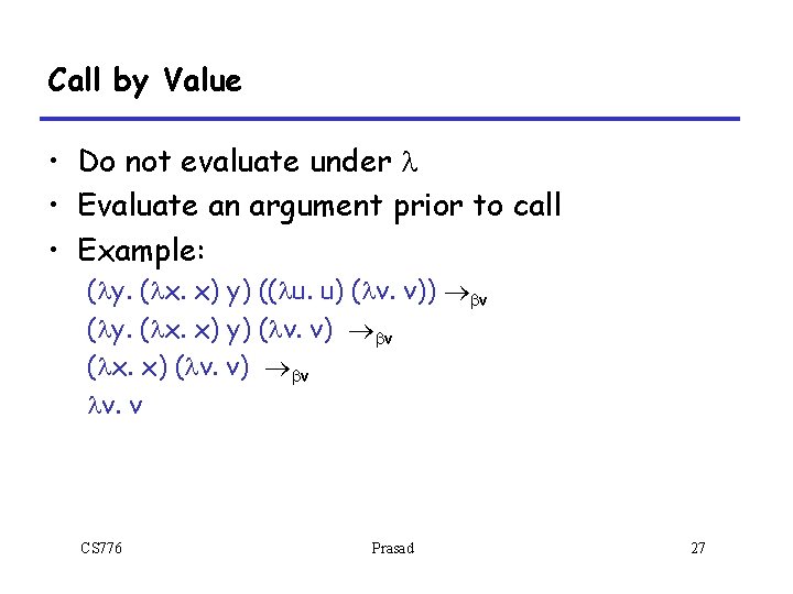
Call by Value • Do not evaluate under l • Evaluate an argument prior to call • Example: (ly. (lx. x) y) ((lu. u) (lv. v)) ®bv (ly. (lx. x) y) (lv. v) ®bv (lx. x) (lv. v) ®bv lv. v CS 776 Prasad 27

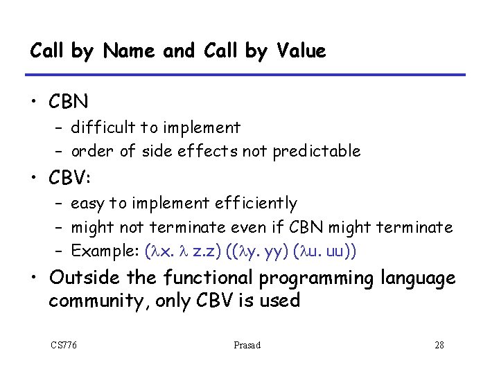
Call by Name and Call by Value • CBN – difficult to implement – order of side effects not predictable • CBV: – easy to implement efficiently – might not terminate even if CBN might terminate – Example: (lx. l z. z) ((ly. yy) (lu. uu)) • Outside the functional programming language community, only CBV is used CS 776 Prasad 28

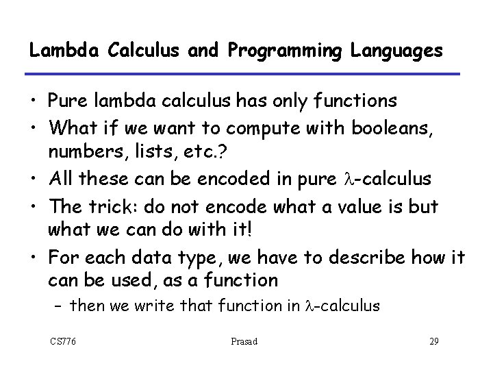
Lambda Calculus and Programming Languages • Pure lambda calculus has only functions • What if we want to compute with booleans, numbers, lists, etc. ? • All these can be encoded in pure l-calculus • The trick: do not encode what a value is but what we can do with it! • For each data type, we have to describe how it can be used, as a function – then we write that function in l-calculus CS 776 Prasad 29

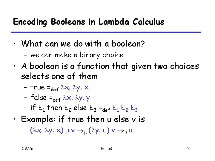
Encoding Booleans in Lambda Calculus • What can we do with a boolean? – we can make a binary choice • A boolean is a function that given two choices selects one of them – true =def lx. ly. x – false =def lx. ly. y – if E 1 then E 2 else E 3 =def E 1 E 2 E 3 • Example: if true then u else v is (lx. ly. x) u v ®b (ly. u) v ®b u CS 776 Prasad 30

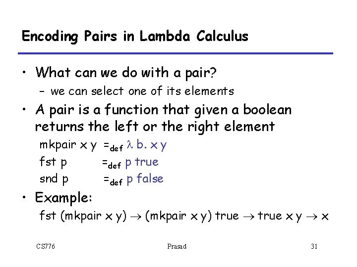
Encoding Pairs in Lambda Calculus • What can we do with a pair? – we can select one of its elements • A pair is a function that given a boolean returns the left or the right element mkpair x y =def l b. x y fst p =def p true snd p =def p false • Example: fst (mkpair x y) ® (mkpair x y) true ® true x y ® x CS 776 Prasad 31

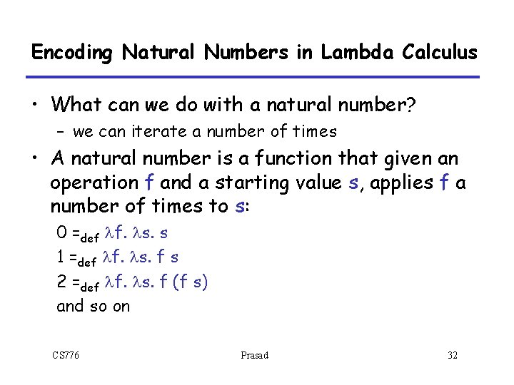
Encoding Natural Numbers in Lambda Calculus • What can we do with a natural number? – we can iterate a number of times • A natural number is a function that given an operation f and a starting value s, applies f a number of times to s: 0 =def lf. ls. s 1 =def lf. ls. f s 2 =def lf. ls. f (f s) and so on CS 776 Prasad 32

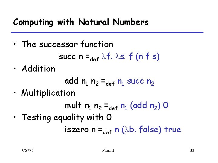
Computing with Natural Numbers • The successor function succ n =def lf. ls. f (n f s) • Addition add n 1 n 2 =def n 1 succ n 2 • Multiplication mult n 1 n 2 =def n 1 (add n 2) 0 • Testing equality with 0 iszero n =def n (lb. false) true CS 776 Prasad 33

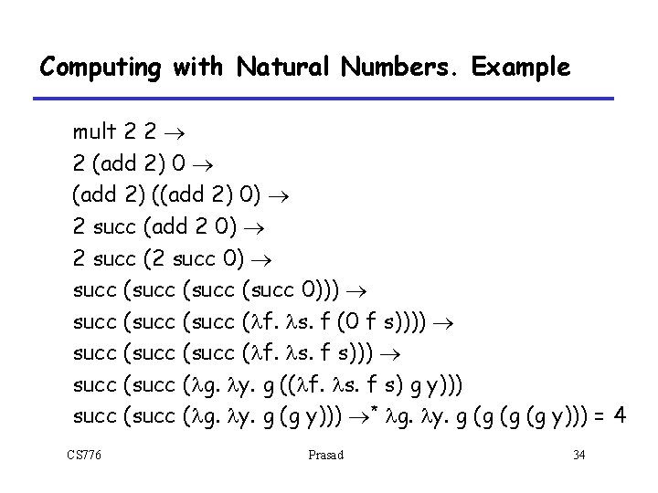
Computing with Natural Numbers. Example mult 2 2 ® 2 (add 2) 0 ® (add 2) ((add 2) 0) ® 2 succ (add 2 0) ® 2 succ (2 succ 0) ® succ (succ 0))) ® succ (succ (lf. ls. f (0 f s)))) ® succ (succ (lf. ls. f s))) ® succ (lg. ly. g ((lf. ls. f s) g y))) succ (lg. ly. g (g y))) ®* lg. ly. g (g (g (g y))) = 4 CS 776 Prasad 34

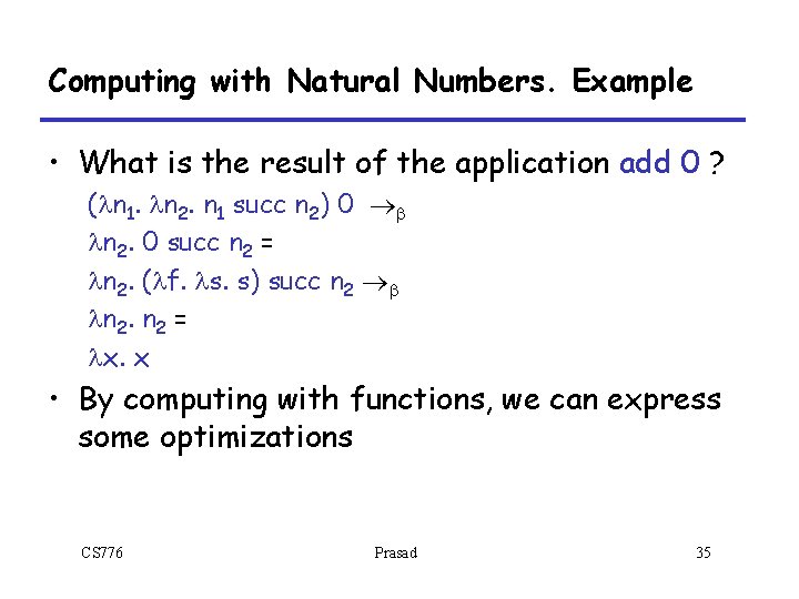
Computing with Natural Numbers. Example • What is the result of the application add 0 ? (ln 1. ln 2. n 1 succ n 2) 0 ®b ln 2. 0 succ n 2 = ln 2. (lf. ls. s) succ n 2 ®b ln 2. n 2 = lx. x • By computing with functions, we can express some optimizations CS 776 Prasad 35

Expressiveness of Lambda Calculus • The l-calculus can express – data types (integers, booleans, lists, trees, etc. ) – branching (using booleans) – recursion • This is enough to encode Turing machines • Encodings are fun • But programming in pure l-calculus is painful – we will add constants (0, 1, 2, …, true, false, if-then -else, etc. ) – and we will add types CS 776 Prasad 36