Foundations of Cryptography Lecture 6 pseudorandom generators hardcore

Foundations of Cryptography Lecture 6: pseudo-random generators, hardcore predicate, Goldreich-Levin Theorem, Next-bit unpredictability. Lecturer: Moni Naor

Recap of last week’s lecture • Signature Scheme definition – Existentially unforgeable against an adaptive chosen message attack • Construction from UOWHFs • Other paradigms for obtaining signature schemes – Trapdoor permutations • Encryption – Desirable properties – One-time pad • Cryptographic pseudo-randomness – Statistical difference – Hardocre predicates

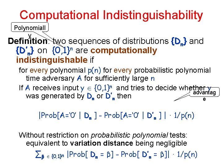
Computational Indistinguishability Polynomiall y Definition: two sequences of distributions {Dn} and {D’n} on {0, 1}n are computationally indistinguishable if for every polynomial p(n) for every probabilistic polynomial time adversary A for sufficiently large n If A receives input y {0, 1}n and tries to decide whether y advantag was generated by Dn or D’n then e |Prob[A=‘ 0’ | Dn ] - Prob[A=‘ 0’ | D’n ] | · 1/p(n) Without restriction on probabilistic polynomial tests: equivalent to variation distance being negligible ∑β {0, 1}n |Prob[ Dn = β] - Prob[ D’n = β]| · 1/p(n)

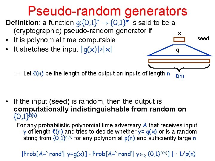
Pseudo-random generators Definition: a function g: {0, 1}* → {0, 1}* is said to be a (cryptographic) pseudo-random generator if x • It is polynomial time computable g • It stretches the input |g(x)|>|x| – Let ℓ(n) be the length of the output on inputs of length n ℓ(n) • If the input (seed) is random, then the output is computationally indistinguishable from random on {0, 1}ℓ(n) For any probabilistic polynomial time adversary A that receives input y of length ℓ(n) and tries to decide whether y= g(x) or is a random string from {0, 1}ℓ(n) for any polynomial p(n) and sufficiently large n |Prob[A=`rand’| y=g(x)] - Prob[A=`rand’| y R {0, 1}ℓ(n)] | · 1/p(n) seed

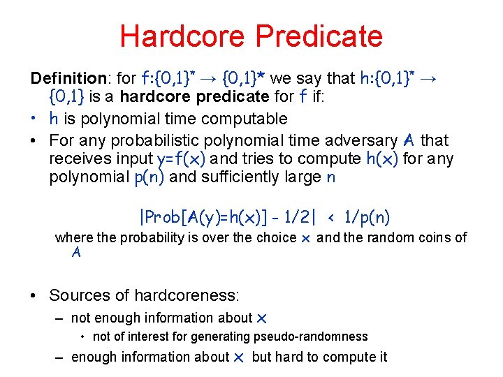
Hardcore Predicate Definition: for f: {0, 1}* → {0, 1}* we say that h: {0, 1}* → {0, 1} is a hardcore predicate for f if: • h is polynomial time computable • For any probabilistic polynomial time adversary A that receives input y=f(x) and tries to compute h(x) for any polynomial p(n) and sufficiently large n |Prob[A(y)=h(x)] - 1/2| < 1/p(n) where the probability is over the choice x and the random coins of A • Sources of hardcoreness: – not enough information about x • not of interest for generating pseudo-randomness – enough information about x but hard to compute it

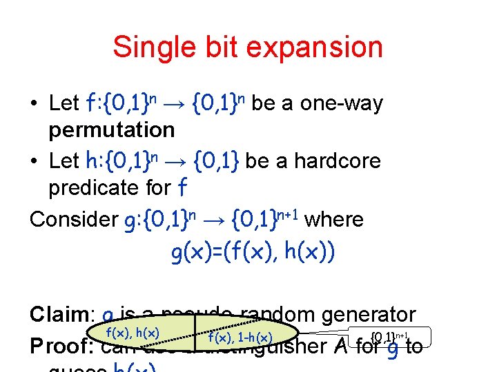
Single bit expansion • Let f: {0, 1}n → {0, 1}n be a one-way permutation • Let h: {0, 1}n → {0, 1} be a hardcore predicate for f Consider g: {0, 1}n → {0, 1}n+1 where g(x)=(f(x), h(x)) Claim: g is a pseudo-random generator f(x), h(x) f(x), 1 -h(x) {0, 1} Proof: can use a distinguisher A for g to n+1

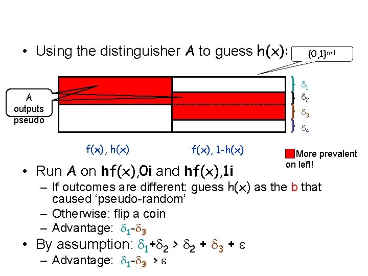
• Using the distinguisher A to guess h(x): {0, 1}n+1 1 2 A outputs pseudo 3 4 f(x), h(x) f(x), 1 -h(x) • Run A on hf(x), 0 i and hf(x), 1 i More prevalent on left! – If outcomes are different: guess h(x) as the b that caused ‘pseudo-random’ – Otherwise: flip a coin – Advantage: 1 - 3 • By assumption: 1+ 2 > 2 + 3 + – Advantage: 1 - 3 >

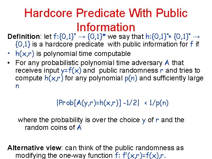
Hardcore Predicate With Public Information Definition: let f: {0, 1}* → {0, 1}* we say that h: {0, 1}*x {0, 1}* → {0, 1} is a hardcore predicate with public information for f if • h(x, r) is polynomial time computable • For any probabilistic polynomial time adversary A that receives input y=f(x) and public randomness r and tries to compute h(x, r) for any polynomial p(n) and sufficiently large n |Prob[A(y, r)=h(x, r)] -1/2| < 1/p(n) where the probability is over the choice y of r and the random coins of A Alternative view: can think of the public randomness as modifying the one-way function f: f’(x, r)=f(x), r.

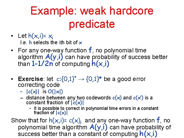
Example: weak hardcore predicate • Let h(x, i)= xi I. e. h selects the ith bit of x • For any one-way function f, no polynomial time algorithm A(y, i) can have probability of success better than 1 -1/2 n of computing h(x, i) • Exercise: let c: {0, 1}* → {0, 1}* be a good error correcting code – |c(x)| is O(|x|) – distance between any two codewords c(x) and c(x’) is a constant fraction of |c(x)| • It is possible to correct in polynomial time errors in a constant fraction of |c(x)| Show that for h(x, i)= c(x)i and any one-way function f, no polynomial time algorithm A(y, i) can have probability of success better than a constant of computing h(x, i)

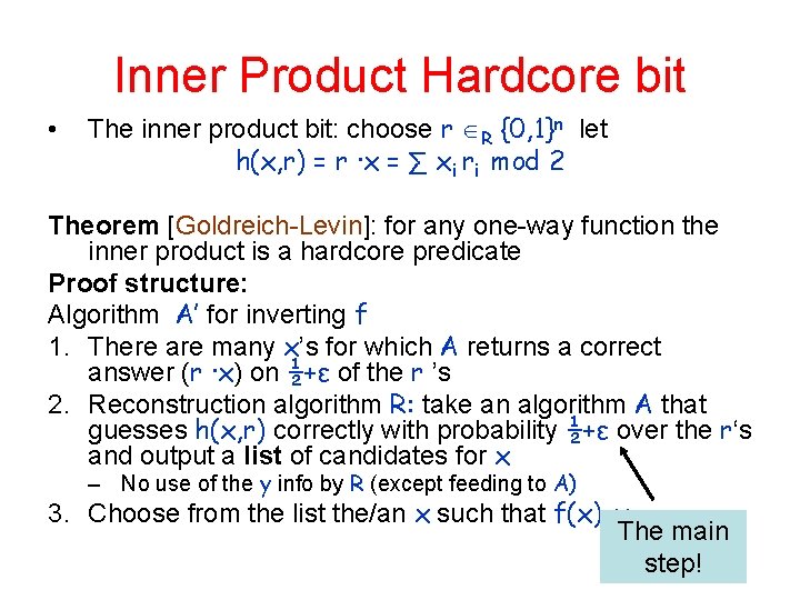
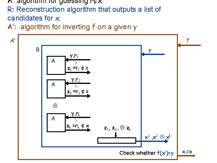
Inner Product Hardcore bit • The inner product bit: choose r R {0, 1}n let h(x, r) = r ∙x = ∑ xi ri mod 2 Theorem [Goldreich-Levin]: for any one-way function the inner product is a hardcore predicate Proof structure: Algorithm A’ for inverting f 1. There are many x’s for which A returns a correct answer (r ∙x) on ½+ε of the r ’s 2. Reconstruction algorithm R: take an algorithm A that guesses h(x, r) correctly with probability ½+ε over the r‘s and output a list of candidates for x – No use of the y info by R (except feeding to A) 3. Choose from the list the/an x such that f(x)=y The main step!

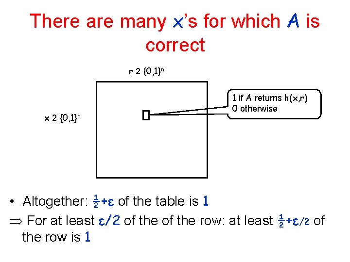
There are many x’s for which A is correct r 2 {0, 1}n x 2 {0, 1}n 1 if A returns h(x, r) 0 otherwise • Altogether: ½+ε of the table is 1 For at least ε/2 of the row: at least ½+ε/2 of the row is 1

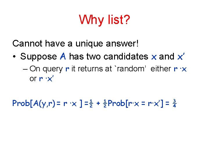
Why list? Cannot have a unique answer! • Suppose A has two candidates x and x’ – On query r it returns at `random’ either r ∙x or r ∙x’ Prob[A(y, r) = r ∙x ] =½ + ½Prob[r∙x = r∙x’] = ¾

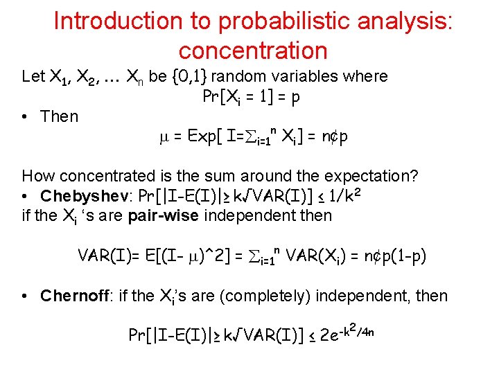
Introduction to probabilistic analysis: concentration Let X 1, X 2, Xn be {0, 1} random variables where Pr[Xi = 1] = p • Then = Exp[ I= i=1 n Xi] = n¢p How concentrated is the sum around the expectation? • Chebyshev: Pr[|I-E(I)|≥ k√VAR(I)] ≤ 1/k 2 if the Xi ‘s are pair-wise independent then VAR(I)= E[(I- )^2] = i=1 n VAR(Xi) = n¢p(1 -p) • Chernoff: if the Xi’s are (completely) independent, then Pr[|I-E(I)|≥ k√VAR(I)] ≤ 2/4 n -k 2 e

A: algorithm for guessing r¢x R: Reconstruction algorithm that outputs a list of candidates for x A’: algorithm for inverting f on a given y y A’ R A A A y y, r 1 ? z 1 =r 1 ¢ x y, r 2 ? z 2 =r 2 ¢ x y, rk ? zk =rk ¢ x z 1 , z 2 , zk x 1 , x 2 xk’ Check whether f(xi)=y xi=x

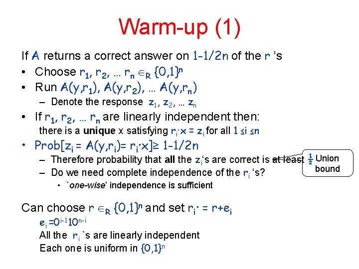
Warm-up (1) If A returns a correct answer on 1 -1/2 n of the r ’s • Choose r 1, r 2, … rn R {0, 1}n • Run A(y, r 1), A(y, r 2), … A(y, rn) – Denote the response z 1, z 2, … zn • If r 1, r 2, … rn are linearly independent then: there is a unique x satisfying ri∙x = zi for all 1 ≤i ≤n • Prob[zi = A(y, ri)= ri∙x]≥ 1 -1/2 n – Therefore probability that all the zi‘s are correct is at least ½ Union bound – Do we need complete independence of the ri ‘s? • `one-wise’ independence is sufficient Can choose r R {0, 1}n and set ri∙ = r+ei ei =0 i-110 n-i All the ri `s are linearly independent Each one is uniform in {0, 1}n

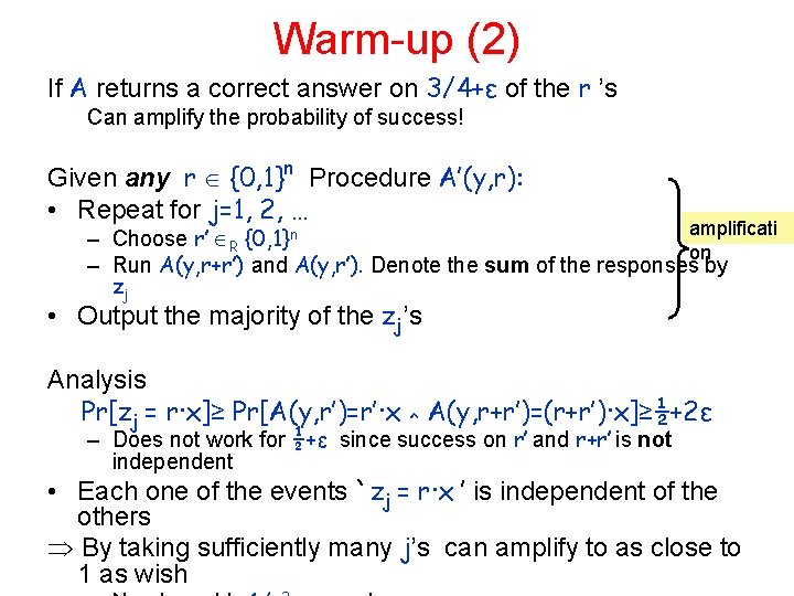
Warm-up (2) If A returns a correct answer on 3/4+ε of the r ’s Can amplify the probability of success! Given any r {0, 1}n Procedure A’(y, r): • Repeat for j=1, 2, … amplificati – Choose r’ R {0, 1}n on – Run A(y, r+r’) and A(y, r’). Denote the sum of the responses by zj • Output the majority of the zj’s Analysis Pr[zj = r∙x]≥ Pr[A(y, r’)=r’∙x ^ A(y, r+r’)=(r+r’)∙x]≥½+2ε – Does not work for ½+ε since success on r’ and r+r’ is not independent • Each one of the events `zj = r∙x ’ is independent of the others By taking sufficiently many j’s can amplify to as close to 1 as wish

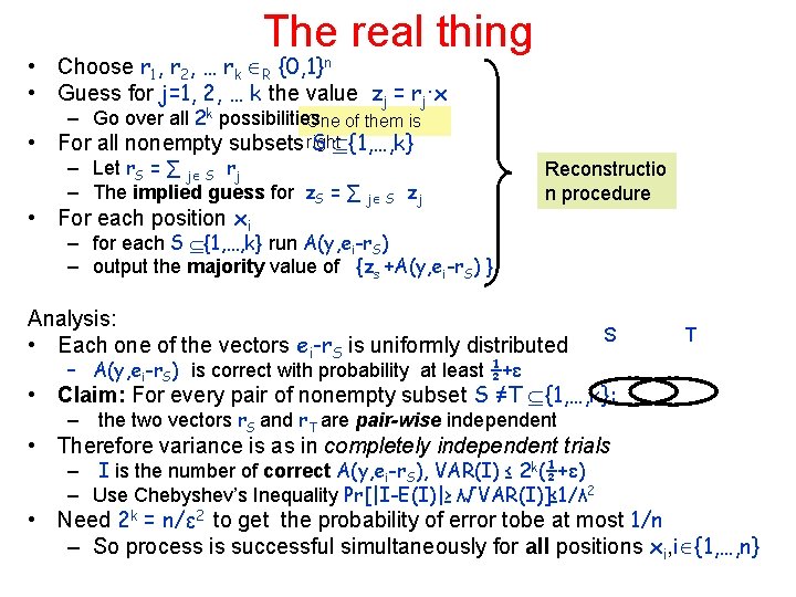
The real thing • Choose r 1, r 2, … rk R {0, 1}n • Guess for j=1, 2, … k the value zj = rj∙x – Go over all 2 k possibilities One of them is • For all nonempty subsets right S {1, …, k} – Let r. S = ∑ j S rj – The implied guess for z. S = ∑ j S zj • For each position xi Reconstructio n procedure – for each S {1, …, k} run A(y, ei-r. S) – output the majority value of {zs +A(y, ei-r. S) } Analysis: • Each one of the vectors ei-r. S is uniformly distributed S T – A(y, ei-r. S) is correct with probability at least ½+ε • Claim: For every pair of nonempty subset S ≠T {1, …, k}: – the two vectors r. S and r. T are pair-wise independent • Therefore variance is as in completely independent trials – I is the number of correct A(y, ei-r. S), VAR(I) ≤ 2 k(½+ε) – Use Chebyshev’s Inequality Pr[|I-E(I)|≥ λ√VAR(I)]≤ 1/λ 2 • Need 2 k = n/ε 2 to get the probability of error tobe at most 1/n – So process is successful simultaneously for all positions xi, i {1, …, n}

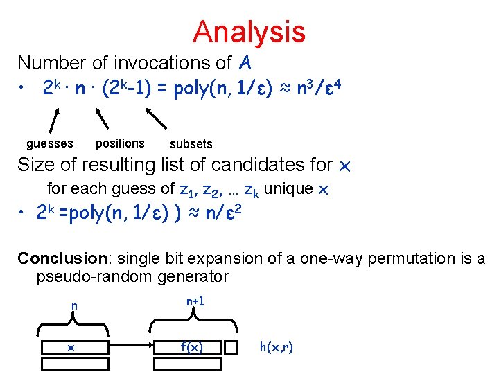
Analysis Number of invocations of A • 2 k ∙ n ∙ (2 k-1) = poly(n, 1/ε) ≈ n 3/ε 4 guesses positions subsets Size of resulting list of candidates for x for each guess of z 1, z 2, … zk unique x • 2 k =poly(n, 1/ε) ) ≈ n/ε 2 Conclusion: single bit expansion of a one-way permutation is a pseudo-random generator n n+1 x f(x) h(x, r)

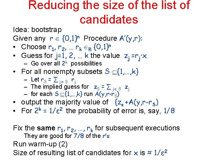
Reducing the size of the list of candidates Idea: bootstrap Given any r {0, 1}n Procedure A’(y, r): • Choose r 1, r 2, … rk R {0, 1}n • Guess for j=1, 2, … k the value zj =rj∙x – Go over all 2 k possibilities • For all nonempty subsets S {1, …, k} – Let r. S = ∑ j S rj – The implied guess for z. S = ∑ j S zj – for each S {1, …, k} run A(y, r-r. S) • output the majority value of {zs +A(y, r-r. S) • For 2 k = 1/ε 2 the probability of error is, say, 1/8 Fix the same r 1, r 2, …, rk for subsequent executions They are good for 7/8 of the r’s Run warm-up (2) Size of resulting list of candidates for x is ≈ 1/ε 2

Application: Diffie-Hellman The Diffie-Hellman assumption Let G be a group and g an element in G. Given g, a=gx and b=gy it is hard to find c=gxy for random x and y the probability of a poly-time machine outputting gxy is negligible More accurately: a sequence of groups • Don’t know how to verify whether given c’ is equal to gxy • Exercise: show that under the DH Assumption Given a=gx , b=gy and r {0, 1}n no polynomial time machine can guess r ∙gxy with advantage 1/poly

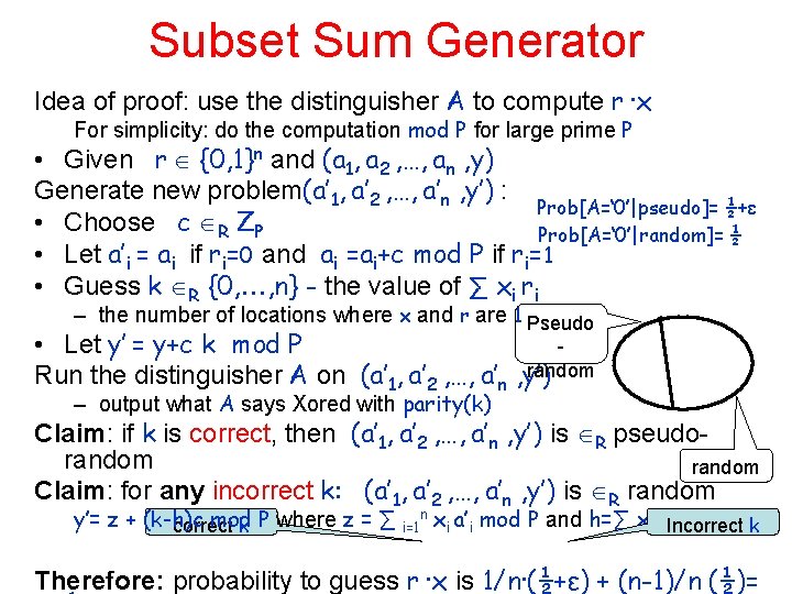
Application: if subset is one-way, then it is a pseudo-random generator • Subset sum problem: given – n numbers 0 ≤ a 1, a 2 , …, an ≤ 2 m – Target sum y – Find subset S⊆ {1, . . . , n} ∑ i S ai, =y • Subset sum one-way function f: {0, 1}mn+n → {0, 1}m+mn f(a 1, a 2 , …, an , x 1, x 2 , …, xn ) = (a 1, a 2 , …, an , ∑ i=1 n xi ai mod 2 m ) If m<n then we get out less bits then we put in. If m>n then we get out more bits then we put in. Theorem: if for m>n subset sum is a one-way function, then it is also a pseudo-random generator

Subset Sum Generator Idea of proof: use the distinguisher A to compute r ∙x For simplicity: do the computation mod P for large prime P • Given r {0, 1}n and (a 1, a 2 , …, an , y) Generate new problem(a’ 1, a’ 2 , …, a’n , y’) : Prob[A=‘ 0’|pseudo]= ½+ε • Choose c R ZP Prob[A=‘ 0’|random]= ½ • Let a’i = ai if ri=0 and ai =ai+c mod P if ri=1 • Guess k R {0, , n} - the value of ∑ xi ri – the number of locations where x and r are 1 Pseudo • Let y’ = y+c k mod P random Run the distinguisher A on (a’ 1, a’ 2 , …, a’n , y’) – output what A says Xored with parity(k) Claim: if k is correct, then (a’ 1, a’ 2 , …, a’n , y’) is R pseudorandom Claim: for any incorrect k: (a’ 1, a’ 2 , …, a’n , y’) is R random y’= z + (k-h)c mod correct k P where z = ∑ i=1 n xi a’i mod P and h=∑ xi r. Incorrect k i Therefore: probability to guess r ∙x is 1/n∙(½+ε) + (n-1)/n (½)=

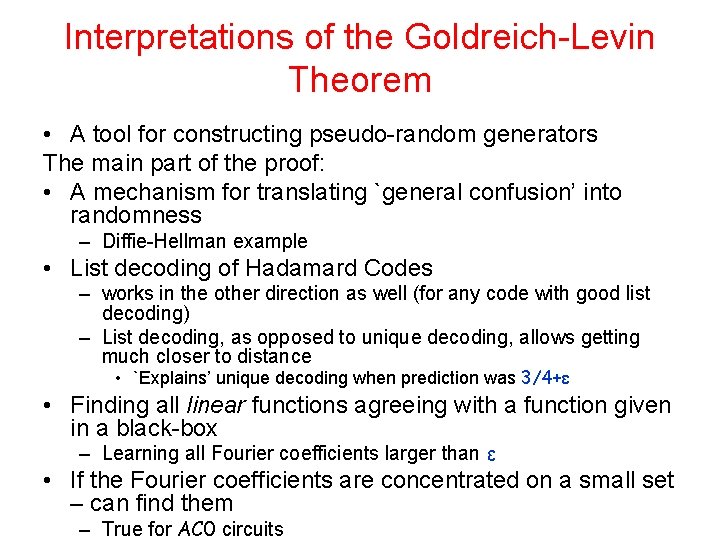
Interpretations of the Goldreich-Levin Theorem • A tool for constructing pseudo-random generators The main part of the proof: • A mechanism for translating `general confusion’ into randomness – Diffie-Hellman example • List decoding of Hadamard Codes – works in the other direction as well (for any code with good list decoding) – List decoding, as opposed to unique decoding, allows getting much closer to distance • `Explains’ unique decoding when prediction was 3/4+ε • Finding all linear functions agreeing with a function given in a black-box – Learning all Fourier coefficients larger than ε • If the Fourier coefficients are concentrated on a small set – can find them – True for AC 0 circuits

Two important techniques for showing pseudo-randomness • Hybrid argument • Next-bit prediction and pseudorandomness

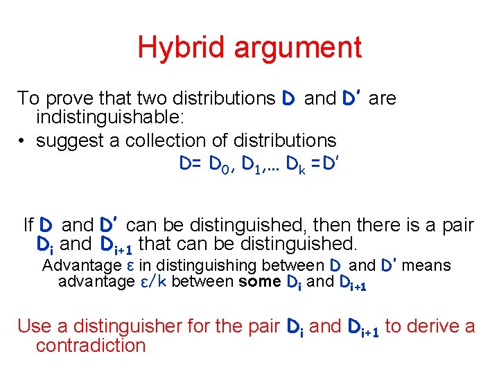
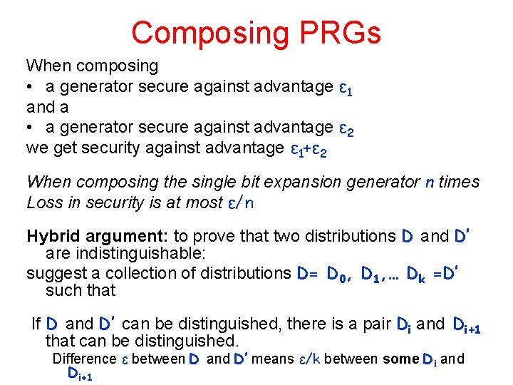
Hybrid argument To prove that two distributions D and D’ are indistinguishable: • suggest a collection of distributions D= D 0, D 1, … Dk =D’ If D and D’ can be distinguished, then there is a pair Di and Di+1 that can be distinguished. Advantage ε in distinguishing between D and D’ means advantage ε/k between some Di and Di+1 Use a distinguisher for the pair Di and Di+1 to derive a contradiction

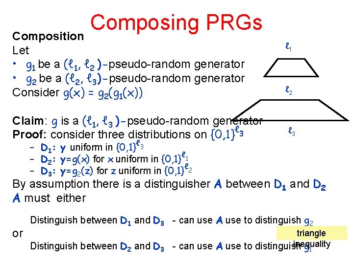
Composing PRGs Composition Let • g 1 be a (ℓ 1, ℓ 2 )-pseudo-random generator • g 2 be a (ℓ 2, ℓ 3)-pseudo-random generator Consider g(x) = g 2(g 1(x)) Claim: g is a (ℓ 1, ℓ 3 )-pseudo-random generator ℓ Proof: consider three distributions on {0, 1} 3 ℓ 1 ℓ 2 ℓ 3 – D 1: y uniform in {0, 1}ℓ 3 ℓ – D 2: y=g(x) for x uniform in {0, 1} 1 – D 3: y=g 2(z) for z uniform in {0, 1}ℓ 2 By assumption there is a distinguisher A between D 1 and D 2 A must either or Distinguish between D 1 and D 3 - can use A use to distinguish g 2 Distinguish between D 2 and D 3 triangle inequality - can use A use to distinguish g 1

Composing PRGs When composing • a generator secure against advantage ε 1 and a • a generator secure against advantage ε 2 we get security against advantage ε 1+ε 2 When composing the single bit expansion generator n times Loss in security is at most ε/n Hybrid argument: to prove that two distributions D and D’ are indistinguishable: suggest a collection of distributions D= D 0, D 1, … Dk =D’ such that If D and D’ can be distinguished, there is a pair Di and Di+1 that can be distinguished. Difference ε between D and D’ means ε/k between some Di and Di+1

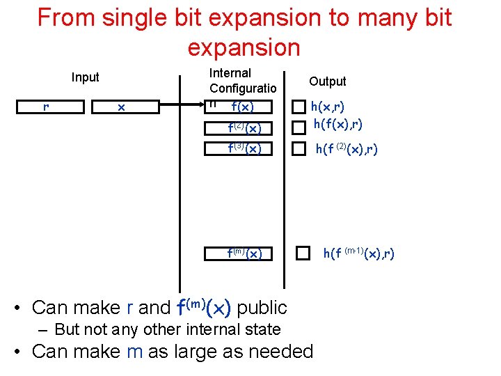
From single bit expansion to many bit expansion Input r x Internal Configuratio n f(x) f(2)(x) Output h(x, r) h(f(x), r) f(3)(x) f(m)(x) • Can make r and f(m)(x) public – But not any other internal state • Can make m as large as needed h(f (2)(x), r) h(f (m-1)(x), r)

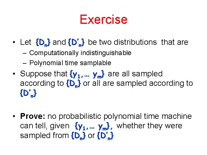
Exercise • Let {Dn} and {D’n} be two distributions that are – Computationally indistinguishable – Polynomial time samplable • Suppose that {y 1, … ym} are all sampled according to {Dn} or all are sampled according to {D’n} • Prove: no probabilistic polynomial time machine can tell, given {y 1, … ym}, whether they were sampled from {Dn} or {D’n}

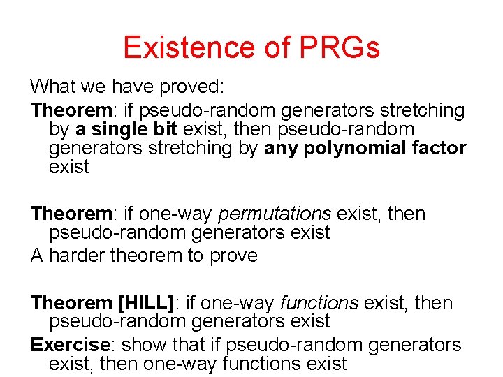
Existence of PRGs What we have proved: Theorem: if pseudo-random generators stretching by a single bit exist, then pseudo-random generators stretching by any polynomial factor exist Theorem: if one-way permutations exist, then pseudo-random generators exist A harder theorem to prove Theorem [HILL]: if one-way functions exist, then pseudo-random generators exist Exercise: show that if pseudo-random generators exist, then one-way functions exist

Two important techniques for showing pseudo-randomness • Hybrid argument • Next-bit prediction and pseudorandomness

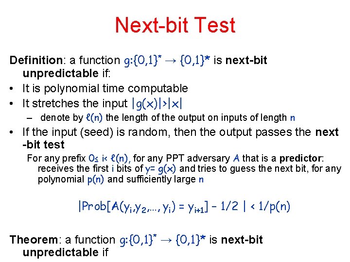
Next-bit Test Definition: a function g: {0, 1}* → {0, 1}* is next-bit unpredictable if: • It is polynomial time computable • It stretches the input |g(x)|>|x| – denote by ℓ(n) the length of the output on inputs of length n • If the input (seed) is random, then the output passes the next -bit test For any prefix 0≤ i< ℓ(n), for any PPT adversary A that is a predictor: receives the first i bits of y= g(x) and tries to guess the next bit, for any polynomial p(n) and sufficiently large n |Prob[A(yi, y 2, …, yi) = yi+1] – 1/2 | < 1/p(n) Theorem: a function g: {0, 1}* → {0, 1}* is next-bit unpredictable if

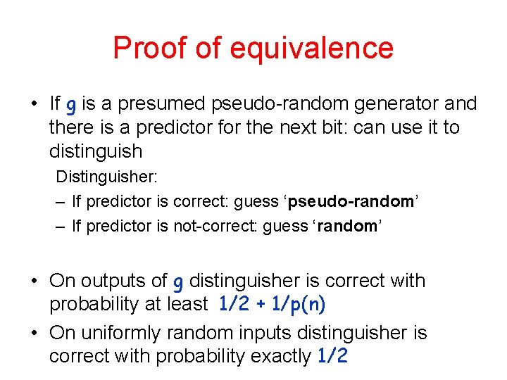
Proof of equivalence • If g is a presumed pseudo-random generator and there is a predictor for the next bit: can use it to distinguish Distinguisher: – If predictor is correct: guess ‘pseudo-random’ – If predictor is not-correct: guess ‘random’ • On outputs of g distinguisher is correct with probability at least 1/2 + 1/p(n) • On uniformly random inputs distinguisher is correct with probability exactly 1/2

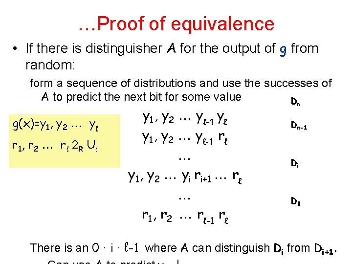
…Proof of equivalence • If there is distinguisher A for the output of g from random: form a sequence of distributions and use the successes of A to predict the next bit for some value Dn g(x)=y 1, y 2 yℓ r 1, r 2 r ℓ 2 R U ℓ y 1, y 2 yℓ-1 yℓ y 1, y 2 yℓ-1 rℓ y 1, y 2 yi ri+1 rℓ r 1, r 2 rℓ-1 rℓ Dn-1 Di D 0 There is an 0 · i · ℓ-1 where A can distinguish Di from Di+1.

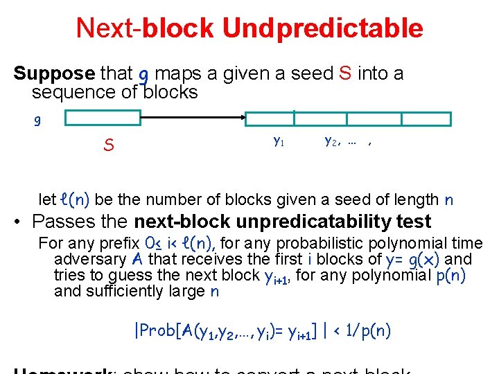
Next-block Undpredictable Suppose that g maps a given a seed S into a sequence of blocks g S y 1 y 2, … , let ℓ(n) be the number of blocks given a seed of length n • Passes the next-block unpredicatability test For any prefix 0≤ i< ℓ(n), for any probabilistic polynomial time adversary A that receives the first i blocks of y= g(x) and tries to guess the next block yi+1, for any polynomial p(n) and sufficiently large n |Prob[A(y 1, y 2, …, yi)= yi+1] | < 1/p(n)

Sources • Goldreich’s Foundations of Cryptography, volumes 1 and 2 • M. Blum and S. Micali, How to Generate Cryptographically Strong Sequences of Pseudo-Random Bits , SIAM J. on Computing, 1984. • O. Goldreich and L. Levin, A Hard-Core Predicate for all One-Way Functions, STOC 1989.