Formulation of Circuit Equations Lecture 2 Alessandra Nardi

Formulation of Circuit Equations Lecture 2 Alessandra Nardi Thanks to Prof. Sangiovanni-Vincentelli and Prof. Newton

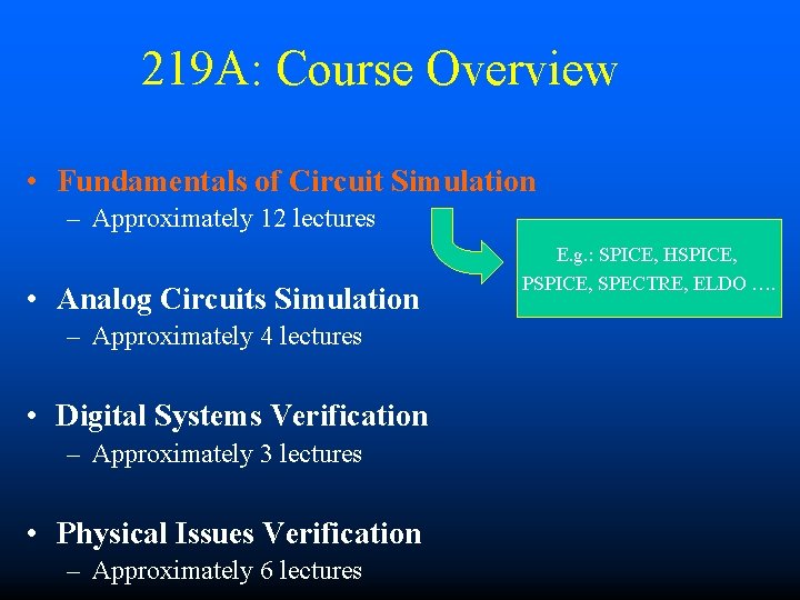
219 A: Course Overview • Fundamentals of Circuit Simulation – Approximately 12 lectures • Analog Circuits Simulation – Approximately 4 lectures • Digital Systems Verification – Approximately 3 lectures • Physical Issues Verification – Approximately 6 lectures E. g. : SPICE, HSPICE, PSPICE, SPECTRE, ELDO ….

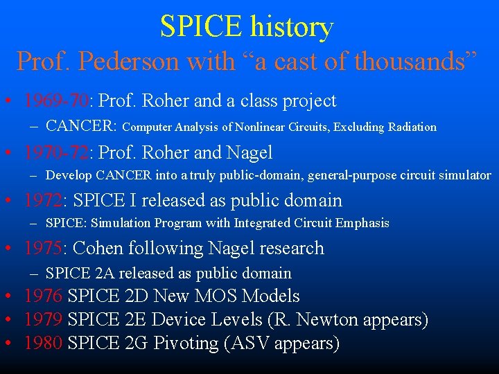
SPICE history Prof. Pederson with “a cast of thousands” • 1969 -70: Prof. Roher and a class project – CANCER: Computer Analysis of Nonlinear Circuits, Excluding Radiation • 1970 -72: Prof. Roher and Nagel – Develop CANCER into a truly public-domain, general-purpose circuit simulator • 1972: SPICE I released as public domain – SPICE: Simulation Program with Integrated Circuit Emphasis • 1975: Cohen following Nagel research – SPICE 2 A released as public domain • 1976 SPICE 2 D New MOS Models • 1979 SPICE 2 E Device Levels (R. Newton appears) • 1980 SPICE 2 G Pivoting (ASV appears)

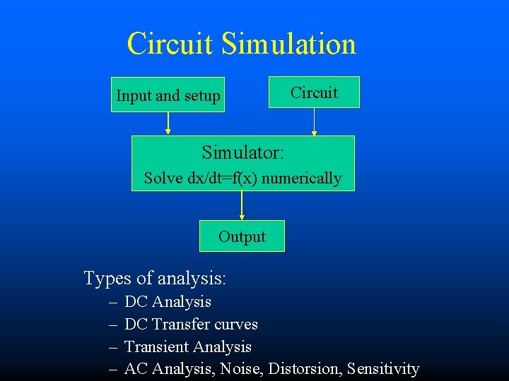
Circuit Simulation Input and setup Circuit Simulator: Solve dx/dt=f(x) numerically Output Types of analysis: – – DC Analysis DC Transfer curves Transient Analysis AC Analysis, Noise, Distorsion, Sensitivity

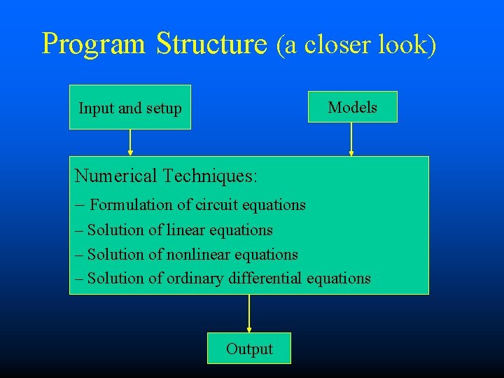
Program Structure (a closer look) Models Input and setup Numerical Techniques: – Formulation of circuit equations – Solution of linear equations – Solution of nonlinear equations – Solution of ordinary differential equations Output

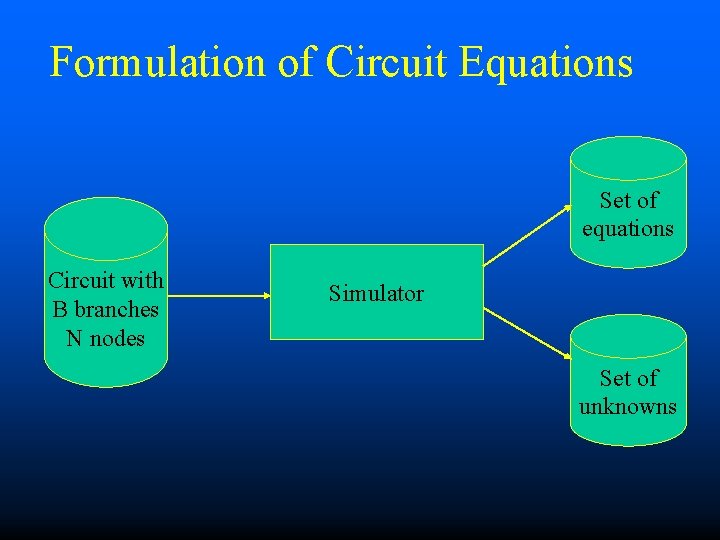
Formulation of Circuit Equations Set of equations Circuit with B branches N nodes Simulator Set of unknowns

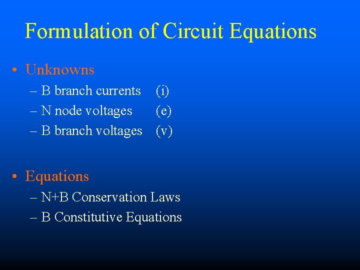
Formulation of Circuit Equations • Unknowns – B branch currents (i) – N node voltages (e) – B branch voltages (v) • Equations – N+B Conservation Laws – B Constitutive Equations

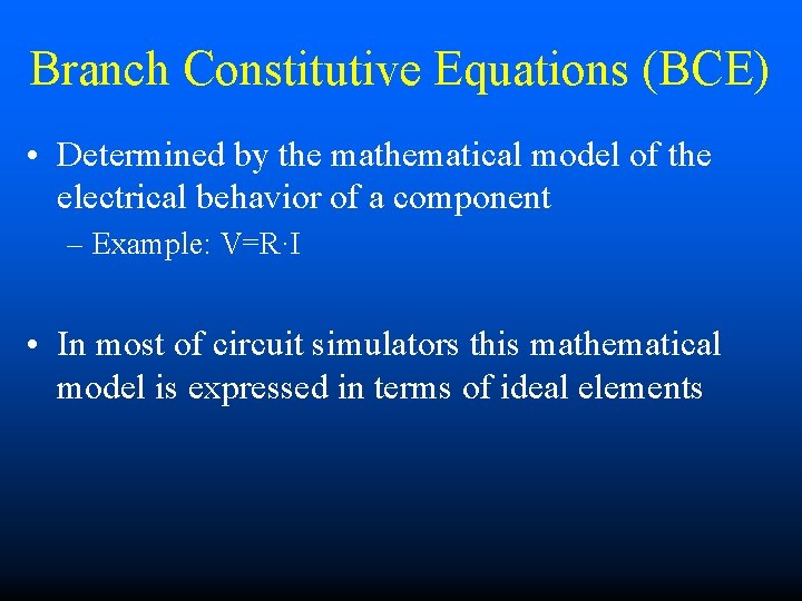
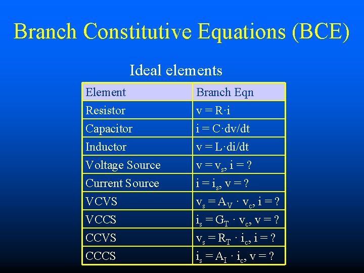
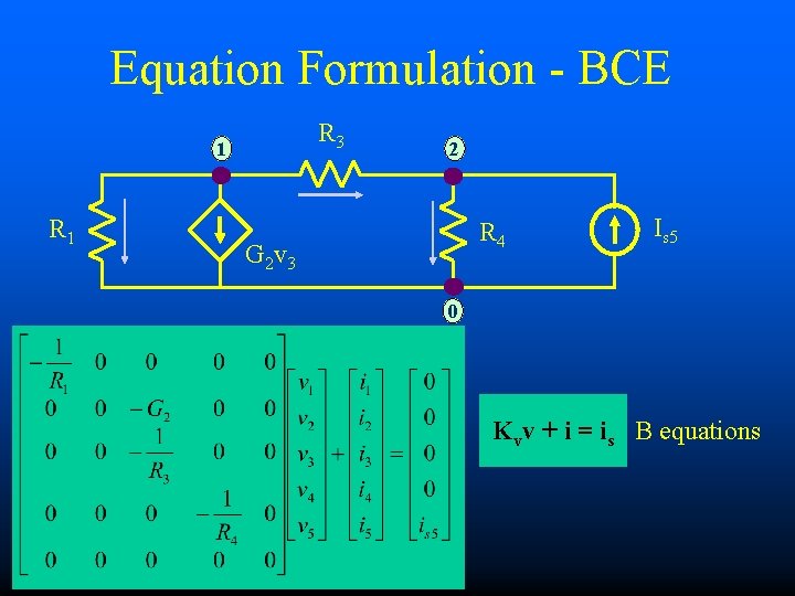
Branch Constitutive Equations (BCE) • Determined by the mathematical model of the electrical behavior of a component – Example: V=R·I • In most of circuit simulators this mathematical model is expressed in terms of ideal elements

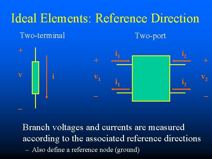
Ideal Elements: Reference Direction Two-terminal Two-port + + v i v 1 i 1 i 2 + v 2 _ _ Branch voltages and currents are measured according to the associated reference directions – Also define a reference node (ground) _

Branch Constitutive Equations (BCE) Ideal elements Element Resistor Capacitor Inductor Branch Eqn v = R·i i = C·dv/dt v = L·di/dt Voltage Source Current Source VCVS VCCS CCVS CCCS v = vs, i = ? i = i s, v = ? vs = AV · vc, i = ? is = GT · vc, v = ? vs = RT · ic, i = ? i s = A I · i c, v = ?

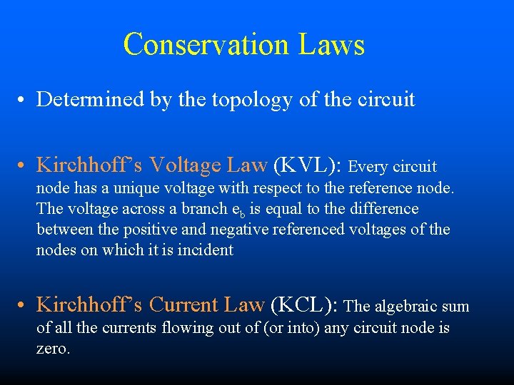
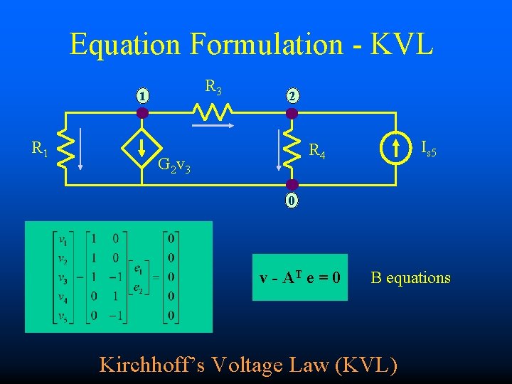
Conservation Laws • Determined by the topology of the circuit • Kirchhoff’s Voltage Law (KVL): Every circuit node has a unique voltage with respect to the reference node. The voltage across a branch eb is equal to the difference between the positive and negative referenced voltages of the nodes on which it is incident • Kirchhoff’s Current Law (KCL): The algebraic sum of all the currents flowing out of (or into) any circuit node is zero.

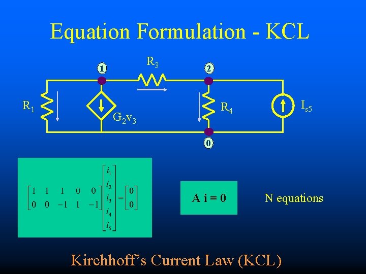
Equation Formulation - KCL R 3 1 R 1 2 Is 5 R 4 G 2 v 3 0 A i = 0 N equations Kirchhoff’s Current Law (KCL)

Equation Formulation - KVL R 3 1 R 1 2 Is 5 R 4 G 2 v 3 0 v - AT e = 0 B equations Kirchhoff’s Voltage Law (KVL)

Equation Formulation - BCE R 3 1 R 1 2 R 4 G 2 v 3 Is 5 0 Kvv + i = is B equations

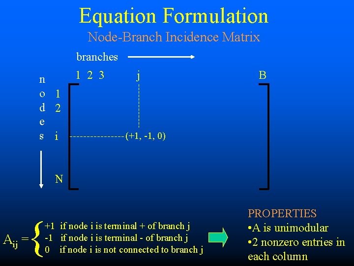
Equation Formulation Node-Branch Incidence Matrix branches n o 1 d 2 e s i 1 2 3 j B (+1, -1, 0) N { Aij = +1 if node i is terminal + of branch j -1 if node i is terminal - of branch j 0 if node i is not connected to branch j PROPERTIES • A is unimodular • 2 nonzero entries in each column

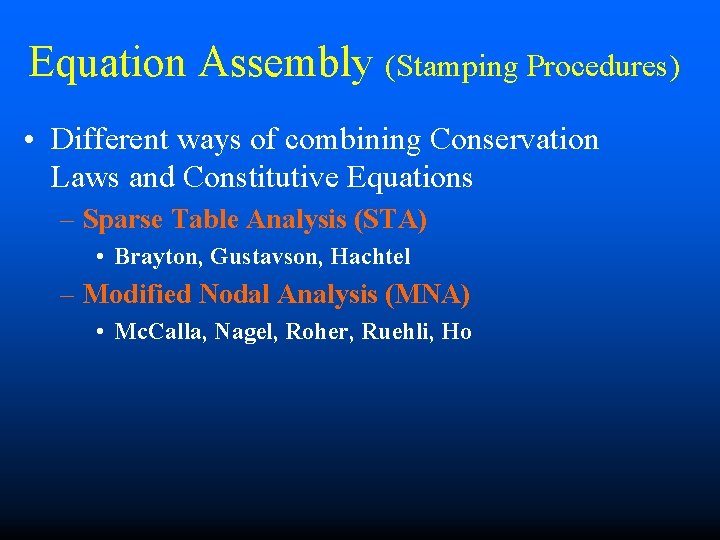
Equation Assembly (Stamping Procedures) • Different ways of combining Conservation Laws and Constitutive Equations – Sparse Table Analysis (STA) • Brayton, Gustavson, Hachtel – Modified Nodal Analysis (MNA) • Mc. Calla, Nagel, Roher, Ruehli, Ho

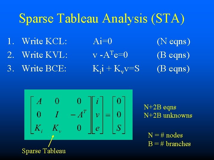
Sparse Tableau Analysis (STA) 1. Write KCL: 2. Write KVL: 3. Write BCE: Ai=0 v -ATe=0 Kii + Kvv=S (N eqns) (B eqns) N+2 B eqns N+2 B unknowns Sparse Tableau N = # nodes B = # branches

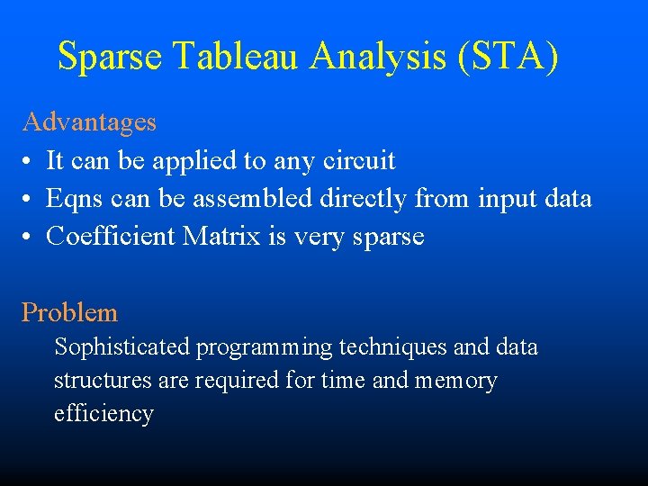
Sparse Tableau Analysis (STA) Advantages • It can be applied to any circuit • Eqns can be assembled directly from input data • Coefficient Matrix is very sparse Problem Sophisticated programming techniques and data structures are required for time and memory efficiency

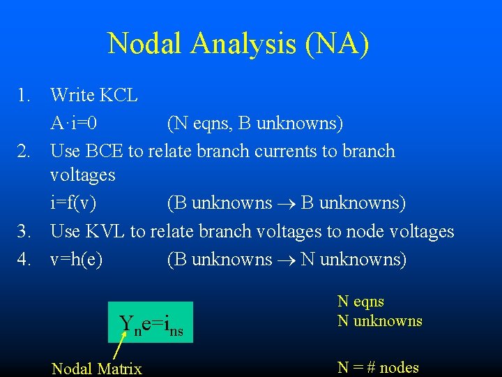
Nodal Analysis (NA) 1. Write KCL A·i=0 (N eqns, B unknowns) 2. Use BCE to relate branch currents to branch voltages i=f(v) (B unknowns B unknowns) 3. Use KVL to relate branch voltages to node voltages 4. v=h(e) (B unknowns N unknowns) Yne=ins Nodal Matrix N eqns N unknowns N = # nodes

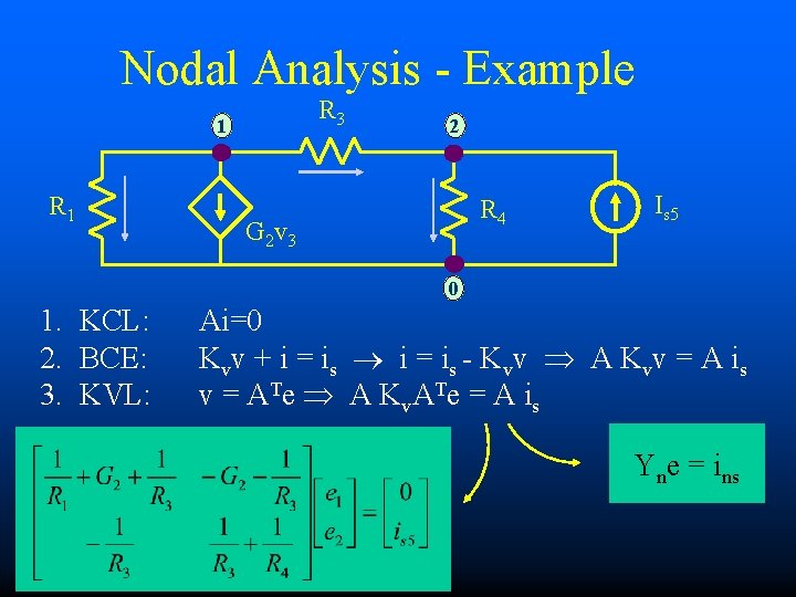
Nodal Analysis - Example R 3 1 R 1 2 R 4 G 2 v 3 Is 5 0 1. KCL: 2. BCE: 3. KVL: Ai=0 Kvv + i = is - Kvv A Kvv = A is v = ATe A Kv. ATe = A is Yne = ins

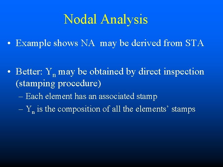
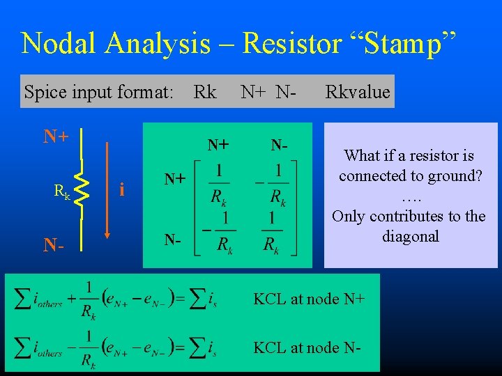
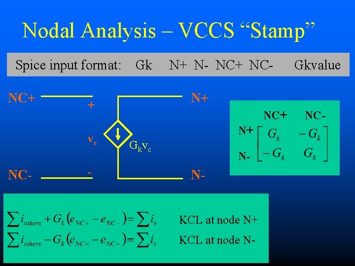
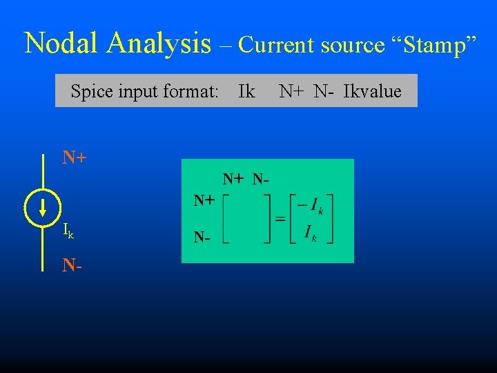
Nodal Analysis • Example shows NA may be derived from STA • Better: Yn may be obtained by direct inspection (stamping procedure) – Each element has an associated stamp – Yn is the composition of all the elements’ stamps

Nodal Analysis – Resistor “Stamp” Spice input format: N+ Rk N- Rk N+ N- N+ N- i N+ N- Rkvalue What if a resistor is connected to ground? …. Only contributes to the diagonal KCL at node N+ KCL at node N-

Nodal Analysis – VCCS “Stamp” Spice input format: NC+ - N+ N- NC+ NC- Gkvalue N+ + vc NC- Gk NC+ NCN+ Gkvc N- NKCL at node N+ KCL at node N-

Nodal Analysis – Current source “Stamp” Spice input format: Ik N+ N+ NN+ Ik N- N- N+ N- Ikvalue

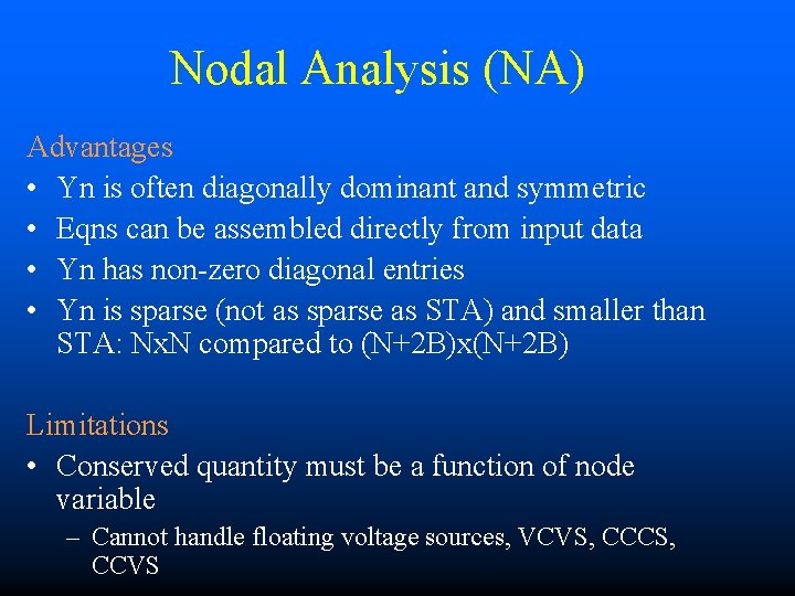
Nodal Analysis (NA) Advantages • Yn is often diagonally dominant and symmetric • Eqns can be assembled directly from input data • Yn has non-zero diagonal entries • Yn is sparse (not as sparse as STA) and smaller than STA: Nx. N compared to (N+2 B)x(N+2 B) Limitations • Conserved quantity must be a function of node variable – Cannot handle floating voltage sources, VCVS, CCCS, CCVS

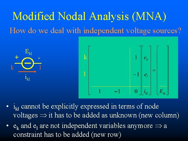
Modified Nodal Analysis (MNA) How do we deal with independent voltage sources? + Ekl k l ikl k l • ikl cannot be explicitly expressed in terms of node voltages it has to be added as unknown (new column) • ek and el are not independent variables anymore a constraint has to be added (new row)

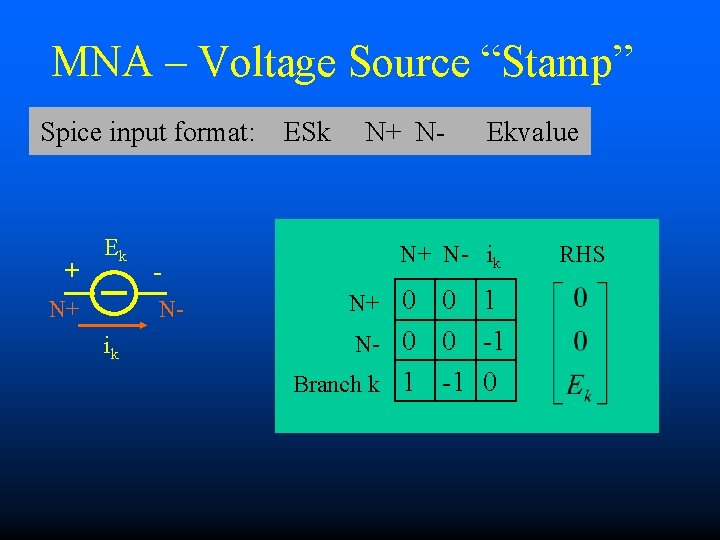
MNA – Voltage Source “Stamp” Spice input format: + Ek N+ N- ik ESk N+ N- Ekvalue N+ N- ik N+ 0 0 1 N- 0 0 -1 Branch k 1 -1 0 RHS

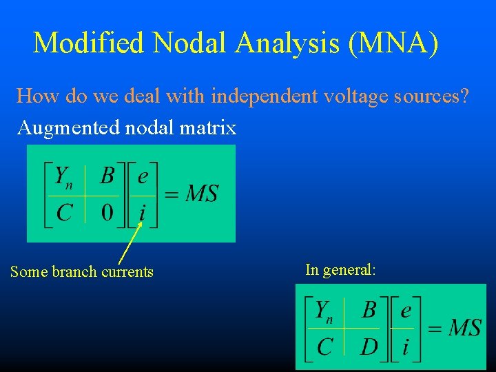
Modified Nodal Analysis (MNA) How do we deal with independent voltage sources? Augmented nodal matrix Some branch currents In general:

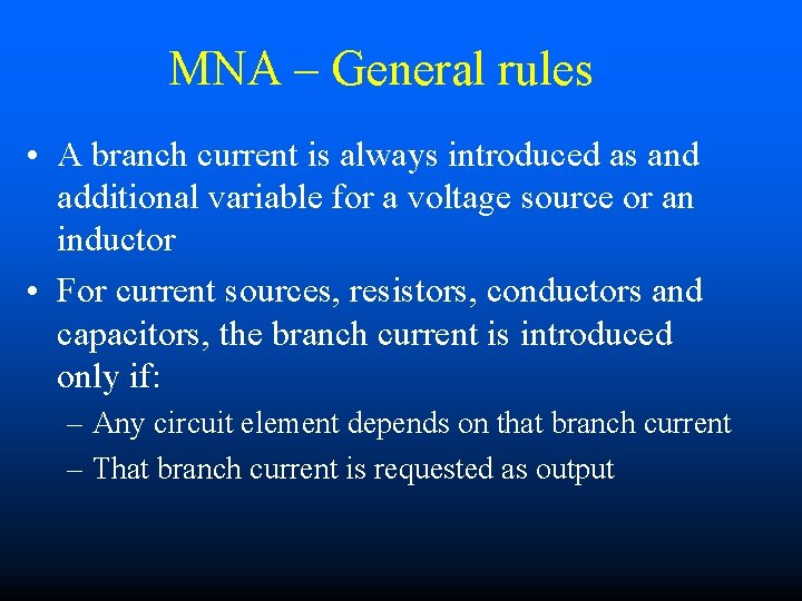
MNA – General rules • A branch current is always introduced as and additional variable for a voltage source or an inductor • For current sources, resistors, conductors and capacitors, the branch current is introduced only if: – Any circuit element depends on that branch current – That branch current is requested as output

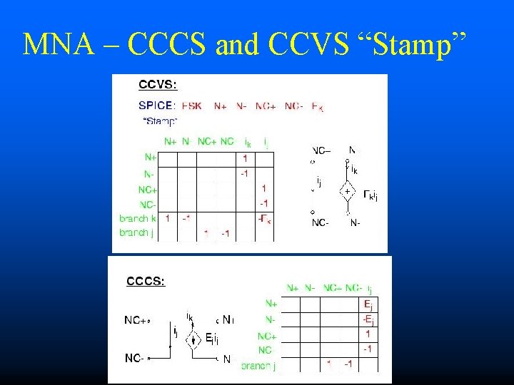
MNA – CCCS and CCVS “Stamp”

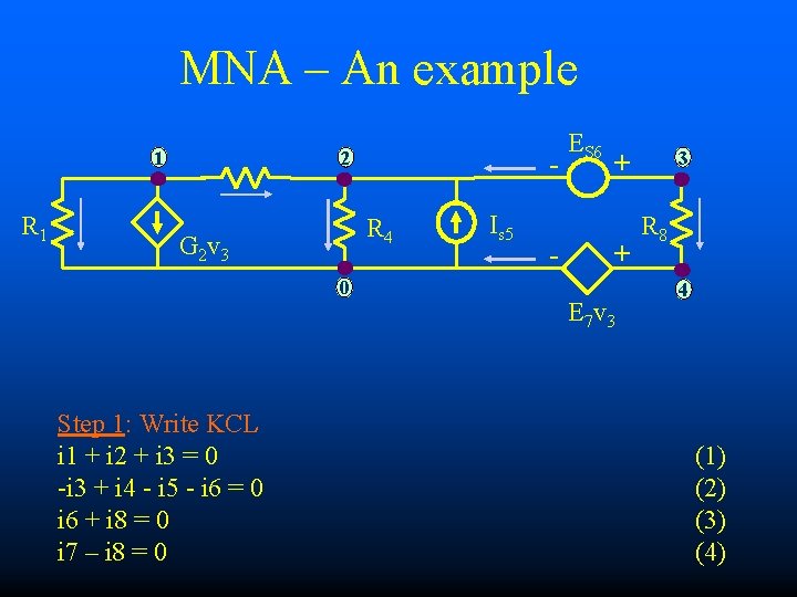
MNA – An example 2 1 R 4 G 2 v 3 0 Step 1: Write KCL i 1 + i 2 + i 3 = 0 -i 3 + i 4 - i 5 - i 6 = 0 i 6 + i 8 = 0 i 7 – i 8 = 0 Is 5 - ES 6 3 + + E 7 v 3 R 8 4 (1) (2) (3) (4)

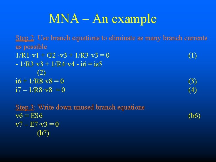
MNA – An example Step 2: Use branch equations to eliminate as many branch currents as possible 1/R 1·v 1 + G 2 ·v 3 + 1/R 3·v 3 = 0 (1) - 1/R 3·v 3 + 1/R 4·v 4 - i 6 = is 5 (2) i 6 + 1/R 8·v 8 = 0 (3) i 7 – 1/R 8·v 8 = 0 (4) Step 3: Write down unused branch equations v 6 = ES 6 v 7 – E 7·v 3 = 0 (b 7) (b 6)

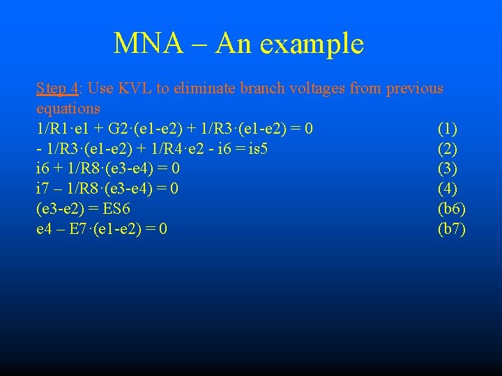
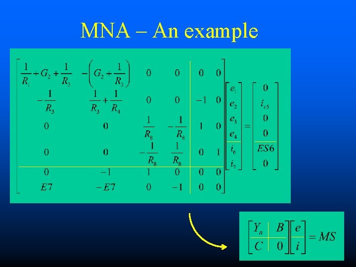
MNA – An example Step 4: Use KVL to eliminate branch voltages from previous equations 1/R 1·e 1 + G 2·(e 1 -e 2) + 1/R 3·(e 1 -e 2) = 0 (1) - 1/R 3·(e 1 -e 2) + 1/R 4·e 2 - i 6 = is 5 (2) i 6 + 1/R 8·(e 3 -e 4) = 0 (3) i 7 – 1/R 8·(e 3 -e 4) = 0 (4) (e 3 -e 2) = ES 6 (b 6) e 4 – E 7·(e 1 -e 2) = 0 (b 7)

MNA – An example

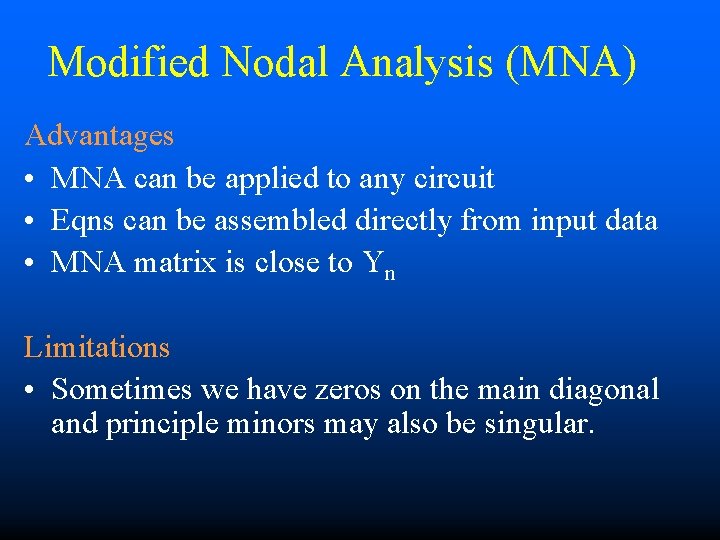
Modified Nodal Analysis (MNA) Advantages • MNA can be applied to any circuit • Eqns can be assembled directly from input data • MNA matrix is close to Yn Limitations • Sometimes we have zeros on the main diagonal and principle minors may also be singular.