Formation et Analyse dImages Session 2 Daniela Hall

Formation et Analyse d’Images Session 2 Daniela Hall 26 September 2005 1

Course Overview • Session 1: – – Overview Human vision Homogenous coordinates Camera models • Session 2: – Tensor notation – Image transformations – Homography computation • Session 3: – Reflection models – Color spaces • Session 4: – Pixel based image analysis • Session 5: – Gaussian filter operators – Scale Space 2

Course overview • Session 6: – Contrast description – Hough transform • Session 7: – Kalman filter • Session 8: – Tracking of regions, pixels, and lines • Session 9: – Stereo vision • Session 10: – Epipolar geometry • Session 11: exercises and questions 3

Trifocal Tensor • A tensor is used in 3 d position estimation with multiple cameras. The (trifocal) tensor encapsulates all the (projective) geometric relations between 3 camera views independent of the scene. • Reference – book: R. Hartley, A. Zisserman: Multiple view geometry in computer vision, Appendix 1, Cambridge University Press, 2000 – Exists on-line http: //www. robots. ox. ac. uk/~vgg/hzbook 1. html 4

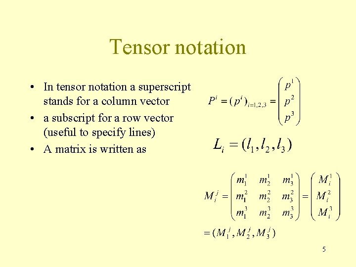
Tensor notation • In tensor notation a superscript stands for a column vector • a subscript for a row vector (useful to specify lines) • A matrix is written as 5

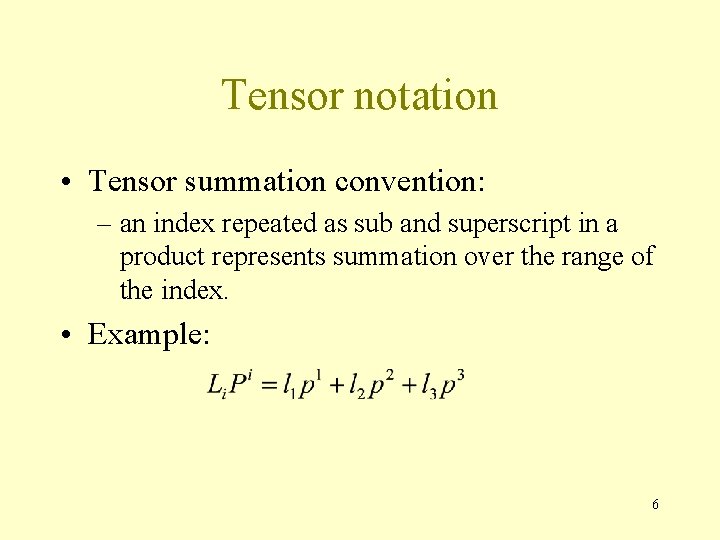
Tensor notation • Tensor summation convention: – an index repeated as sub and superscript in a product represents summation over the range of the index. • Example: 6

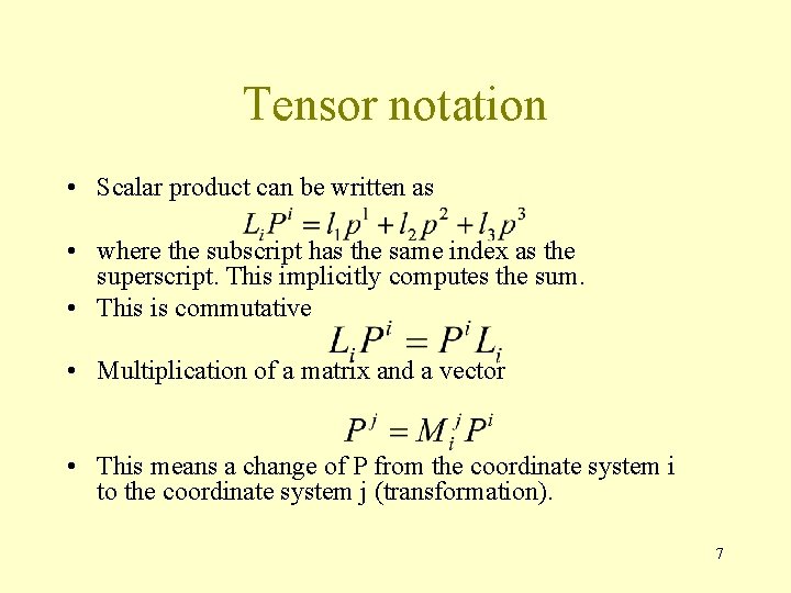
Tensor notation • Scalar product can be written as • where the subscript has the same index as the superscript. This implicitly computes the sum. • This is commutative • Multiplication of a matrix and a vector • This means a change of P from the coordinate system i to the coordinate system j (transformation). 7

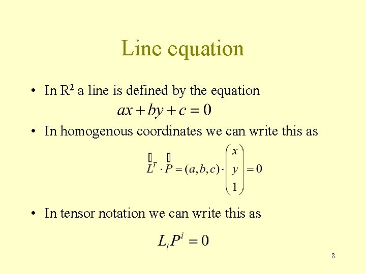
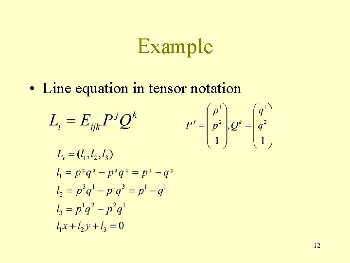
Line equation • In R 2 a line is defined by the equation • In homogenous coordinates we can write this as • In tensor notation we can write this as 8

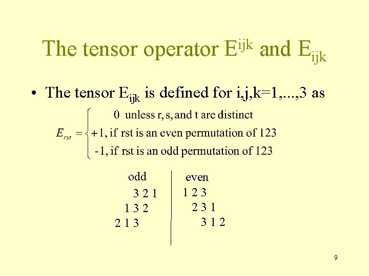
The tensor operator ijk E and Eijk • The tensor Eijk is defined for i, j, k=1, . . . , 3 as odd 321 132 213 even 123 231 312 9

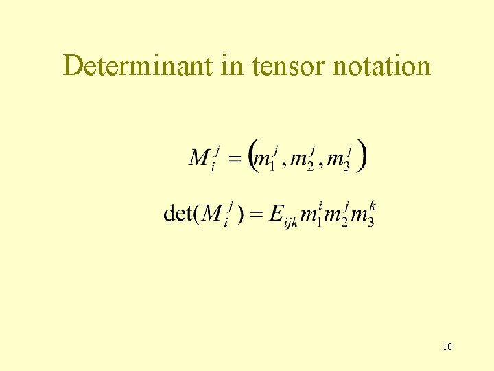
Determinant in tensor notation 10

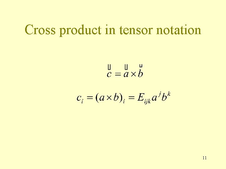
Cross product in tensor notation 11

Example • Line equation in tensor notation 12

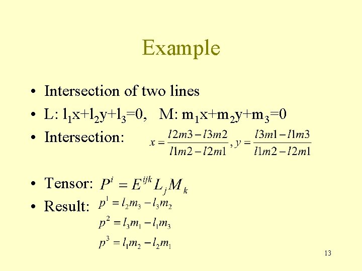
Example • Intersection of two lines • L: l 1 x+l 2 y+l 3=0, M: m 1 x+m 2 y+m 3=0 • Intersection: • Tensor: • Result: 13

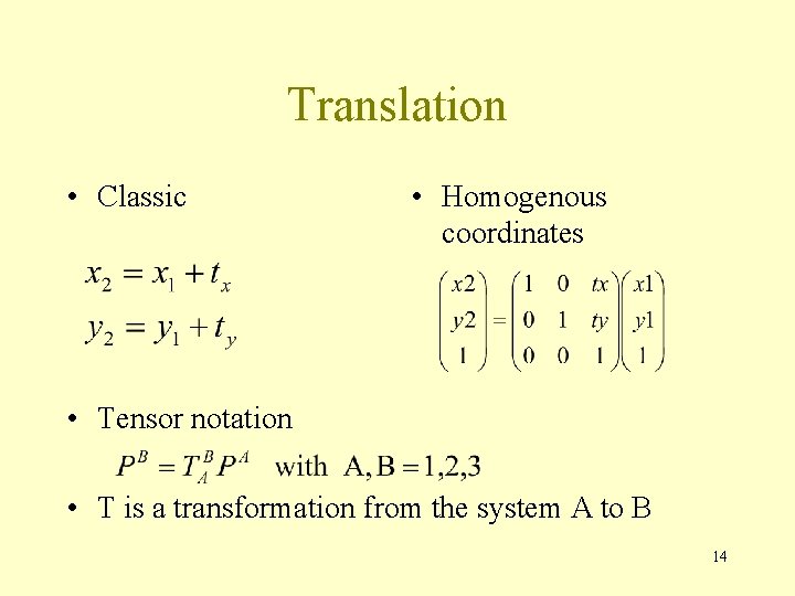
Translation • Classic • Homogenous coordinates • Tensor notation • T is a transformation from the system A to B 14

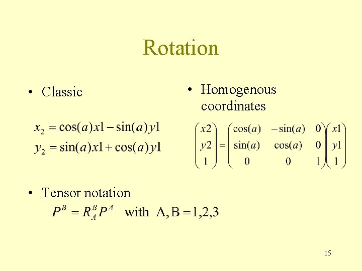
Rotation • Classic • Homogenous coordinates • Tensor notation 15

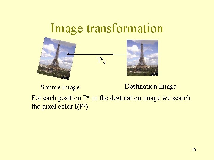
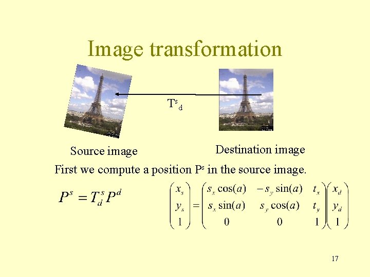
Image transformation T sd Source image Destination image For each position Pd in the destination image we search the pixel color I(Pd). 16

Image transformation T sd Source image Destination image First we compute a position Ps in the source image. 17

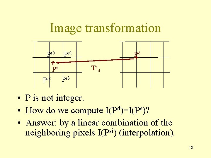
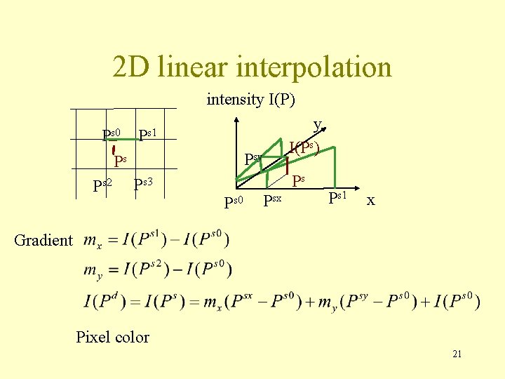
Image transformation Ps 0 Ps 1 T sd Ps Ps 2 Pd Ps 3 • P is not integer. • How do we compute I(Pd)=I(Ps)? • Answer: by a linear combination of the neighboring pixels I(Psi) (interpolation). 18

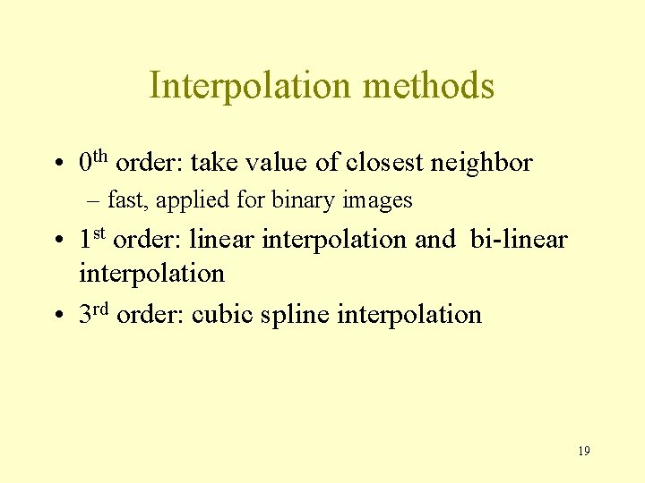
Interpolation methods • 0 th order: take value of closest neighbor – fast, applied for binary images • 1 st order: linear interpolation and bi-linear interpolation • 3 rd order: cubic spline interpolation 19

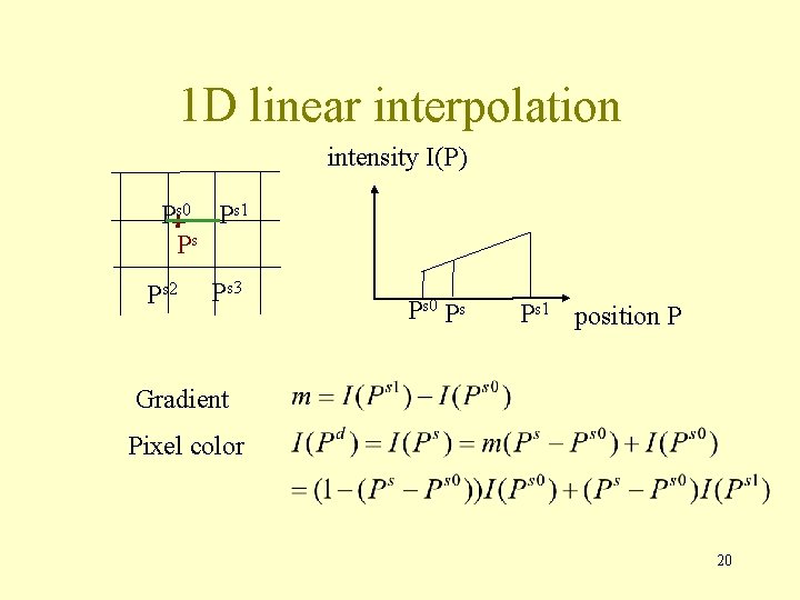
1 D linear interpolation intensity I(P) Ps 0 Ps 1 Ps Ps 2 Ps 3 Ps 0 Ps Ps 1 position P Gradient Pixel color 20

2 D linear interpolation intensity I(P) Ps 0 Ps 1 Psy Ps Ps 2 Ps 3 y I(Ps) Ps Ps 0 Psx Ps 1 x Gradient Pixel color 21

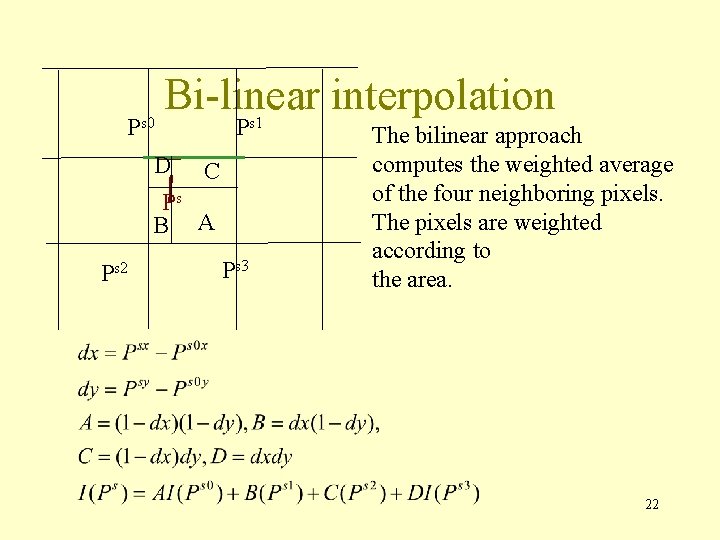
Ps 0 Bi-linear interpolation D Ps 1 C Ps B A Ps 2 Ps 3 The bilinear approach computes the weighted average of the four neighboring pixels. The pixels are weighted according to the area. 22

Higher order interpolation • Cubic spline interpolation takes into account more than only the closest pixels. • Result: more expensive to compute, but image has less artefacts, image is smoother. 23

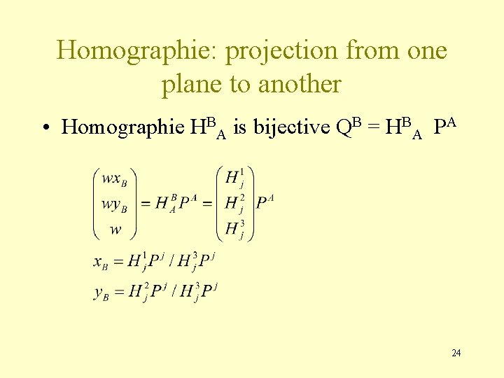
Homographie: projection from one plane to another • Homographie HBA is bijective QB = HBA PA 24

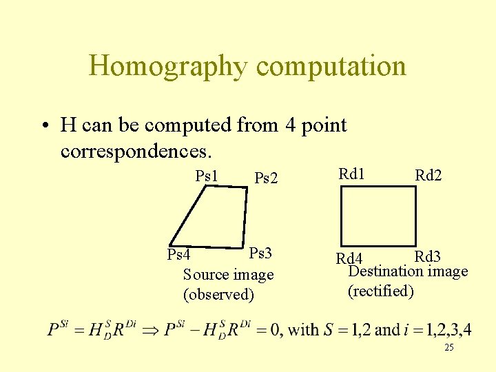
Homography computation • H can be computed from 4 point correspondences. Ps 1 Ps 2 Ps 3 Ps 4 Source image (observed) Rd 1 Rd 2 Rd 3 Rd 4 Destination image (rectified) 25

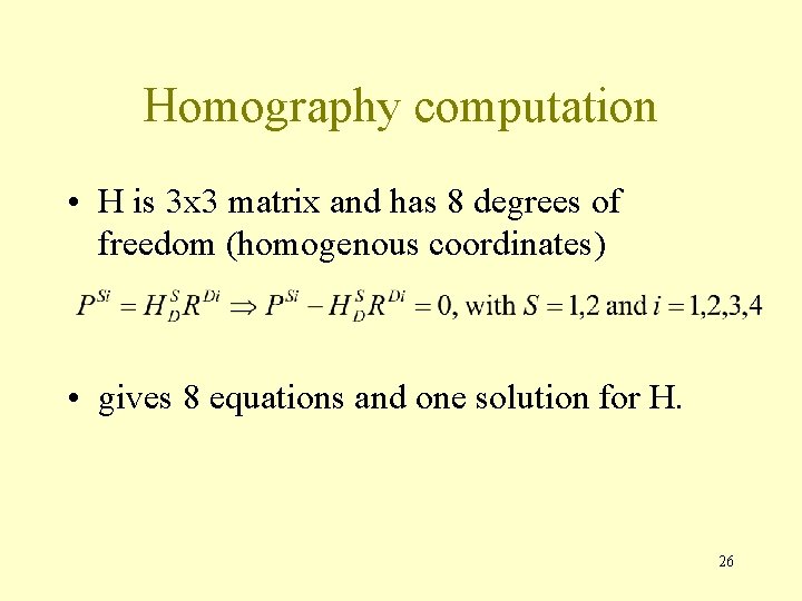
Homography computation • H is 3 x 3 matrix and has 8 degrees of freedom (homogenous coordinates) • gives 8 equations and one solution for H. 26

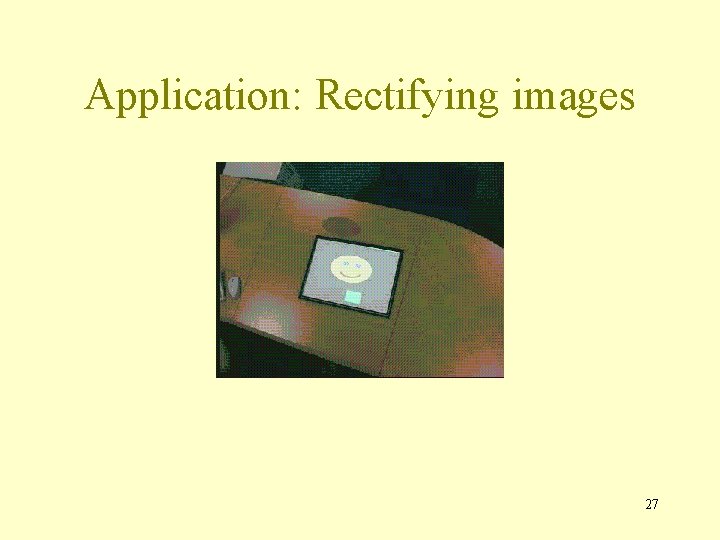
Application: Rectifying images 27

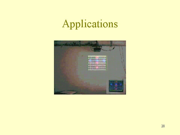
Applications 28