Forecasting What is Forecasting l Process of predicting

Forecasting

What is Forecasting? l Process of predicting a future event l Underlying basis of all business decisions: l l Production Inventory Personnel Facilities

Forecasts by Time Horizon l Short-range forecast l Up to 1 year (usually less than 3 months) l Job scheduling, worker assignments l Medium-range forecast l 3 months to 3 years l Sales & production planning, budgeting l Long-range l 3 forecast years, or more l New product planning, facility location

Long vs. Short Term Forecasting l Long and Medium range forecasts l deal with more comprehensive issues l support management decisions regarding planning and products, plants and processes. l Short-term l usually forecasts employ different methodologies than longer-term forecasting l tend to be more accurate than longer-term forecasts.

Influence of Product Life Cycle Introduction, Growth, Maturity, Decline l Stages of introduction and growth require longer forecasts than maturity and decline l Forecasts useful in projecting l l l Staffing levels, Inventory levels, and Factory capacity as product passes through life cycle stages

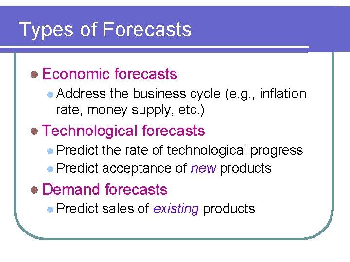
Types of Forecasts l Economic forecasts l Address the business cycle (e. g. , inflation rate, money supply, etc. ) l Technological forecasts l Predict the rate of technological progress l Predict acceptance of new products l Demand l Predict forecasts sales of existing products

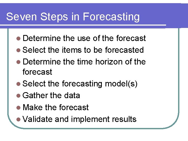
Seven Steps in Forecasting l Determine the use of the forecast l Select the items to be forecasted l Determine the time horizon of the forecast l Select the forecasting model(s) l Gather the data l Make the forecast l Validate and implement results

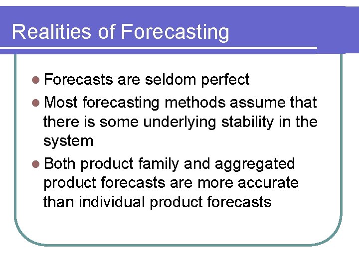
Realities of Forecasting l Forecasts are seldom perfect l Most forecasting methods assume that there is some underlying stability in the system l Both product family and aggregated product forecasts are more accurate than individual product forecasts

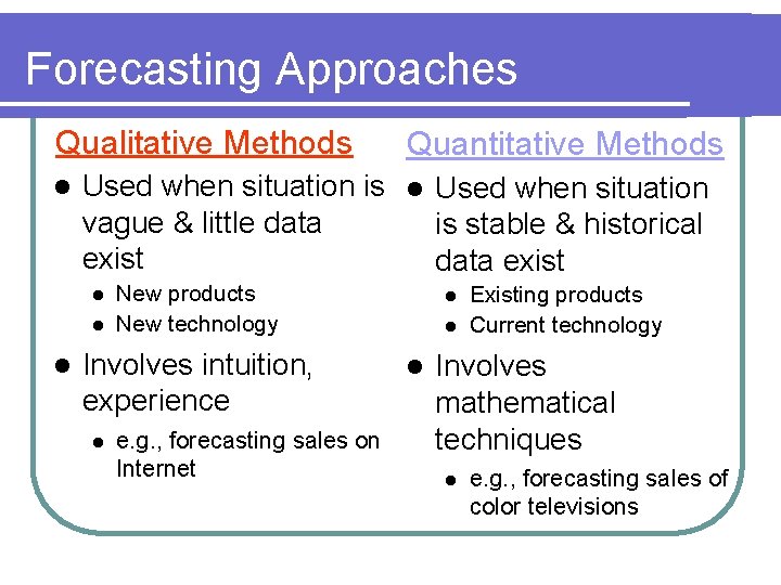
Forecasting Approaches Qualitative Methods l Used when situation is l Used when situation vague & little data is stable & historical exist data exist l l l Quantitative Methods New products New technology Involves intuition, experience l e. g. , forecasting sales on Internet l l l Existing products Current technology Involves mathematical techniques l e. g. , forecasting sales of color televisions

Forecasting Approaches …The reality of all forecasting techniques is that they depend on both subjective and objective inputs… …That is to say that, regardless of the initial approach, all forecasting techniques are a blend of both art and science

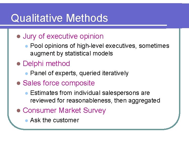
Qualitative Methods l Jury of executive opinion l l Delphi method l l Panel of experts, queried iteratively Sales force composite l l Pool opinions of high-level executives, sometimes augment by statistical models Estimates from individual salespersons are reviewed for reasonableness, then aggregated Consumer Market Survey l Ask the customer

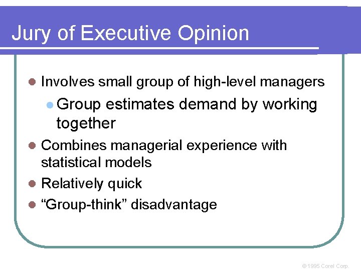
Jury of Executive Opinion l Involves small group of high-level managers l Group estimates demand by working together Combines managerial experience with statistical models l Relatively quick l “Group-think” disadvantage l © 1995 Corel Corp.

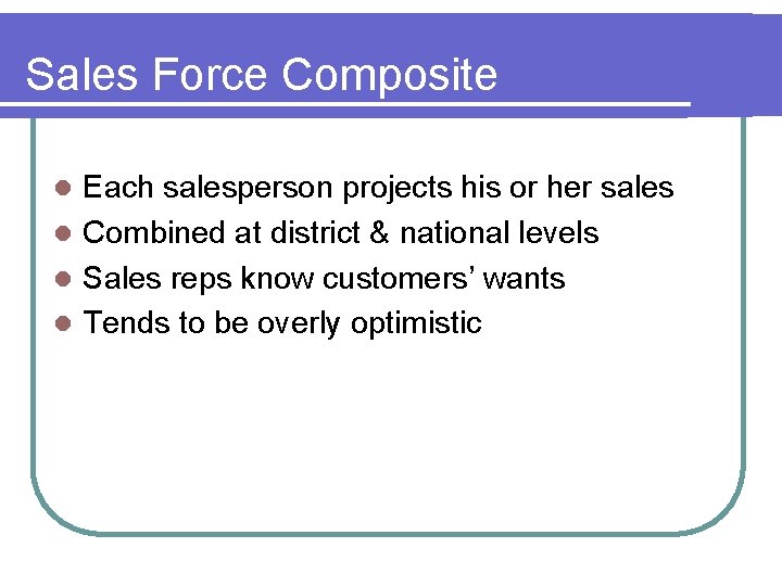
Sales Force Composite Each salesperson projects his or her sales l Combined at district & national levels l Sales reps know customers’ wants l Tends to be overly optimistic l

Delphi Method l Iterative group process l 3 types of people Decision makers l Staff l Respondents l l Reduces ‘group-think’

Consumer Market Survey Ask customers about purchasing plans l What consumers say, and what they actually do are often different l Sometimes difficult to answer l

Quantitative Approaches l Naïve approach l Moving average l Weighted moving average l Exponential smoothing with trend l Trend projection l Seasonally adjusted

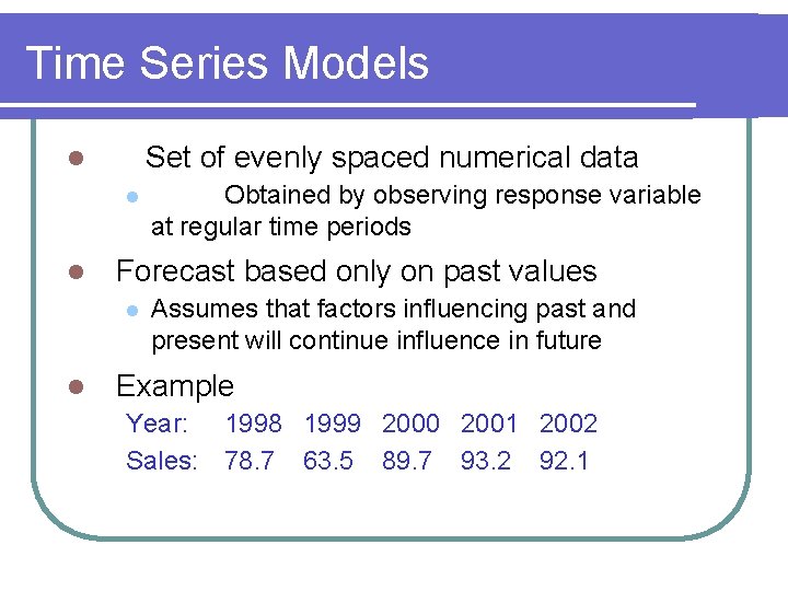
Time Series Models Set of evenly spaced numerical data l l l Forecast based only on past values l l Obtained by observing response variable at regular time periods Assumes that factors influencing past and present will continue influence in future Example Year: 1998 1999 2000 2001 2002 Sales: 78. 7 63. 5 89. 7 93. 2 92. 1

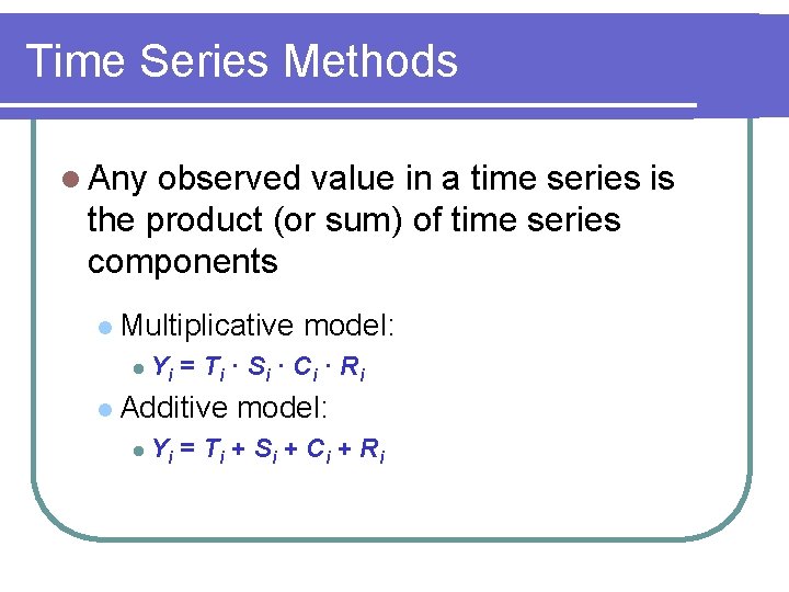
Time Series Methods l Any observed value in a time series is the product (or sum) of time series components l Multiplicative l Yi = T i · S i · Ci · Ri l Additive l Yi model: = T i + S i + Ci + Ri

Time Series Terms Stationary Data l a time series variable exhibiting no significant upward or downward trend over time Nonstationary Data l a time series variable exhibiting a significant upward or downward trend over time Seasonal Data l a time series variable exhibiting a repeating patterns at regular intervals over time

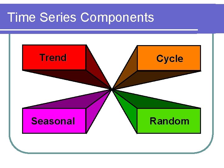
Time Series Components Trend Cycle Seasonal Random

Trend Component l Persistent, overall upward or downward pattern l Due to population, technology etc. l Several years duration

Seasonal Component l Regular pattern of up & down fluctuations l Due to weather, customs, etc. l Occurs within 1 year

Cyclical Component l Repeating up & down movements l Due to interactions of factors influencing economy l Can be anywhere between 2 -30+ years duration

Random Component l Erratic, unsystematic, ‘residual’ fluctuations l Due to random variation or unforeseen events l l Union strike l Tornado Short duration & non-repeating

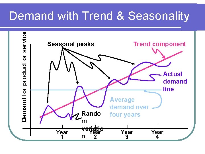
Demand for product or service Demand with Trend & Seasonality Seasonal peaks Trend component Actual demand line Year 1 Rando m variatio Year n 2 Average demand over four years Year 3 Year 4

Time Series Analysis There are many, many different time series techniques l It is usually impossible to know which technique will be best for a particular data set l It is customary to try out several different techniques and select the one that seems to work best l To be an effective time series modeler, you need to keep several time series techniques in your “tool box” l

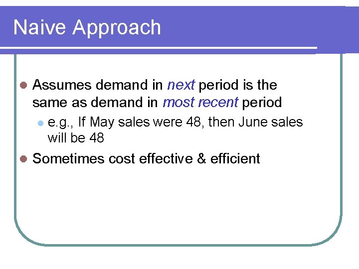
Naive Approach l Assumes demand in next period is the same as demand in most recent period l l e. g. , If May sales were 48, then June sales will be 48 Sometimes cost effective & efficient

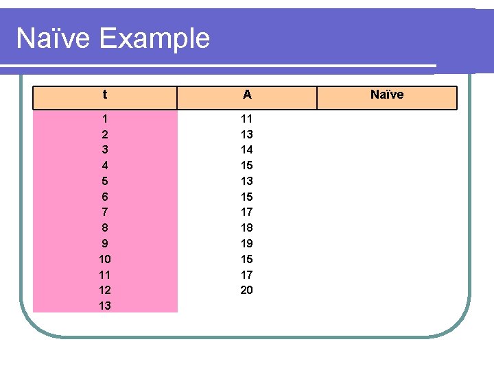
Naïve Example t A 1 2 3 4 5 6 7 8 9 10 11 12 13 11 13 14 15 13 15 17 18 19 15 17 20 Naïve

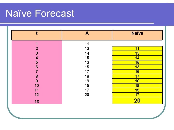
Naïve Forecast t A Naïve 1 2 3 4 5 6 7 8 9 10 11 12 11 13 14 15 13 15 17 18 19 15 17 20 11 13 14 15 13 15 17 18 19 15 17 13 20

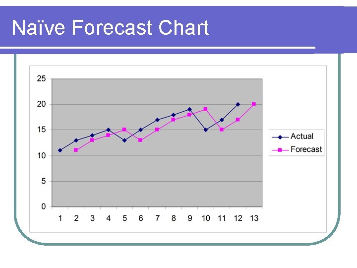
Naïve Forecast Chart

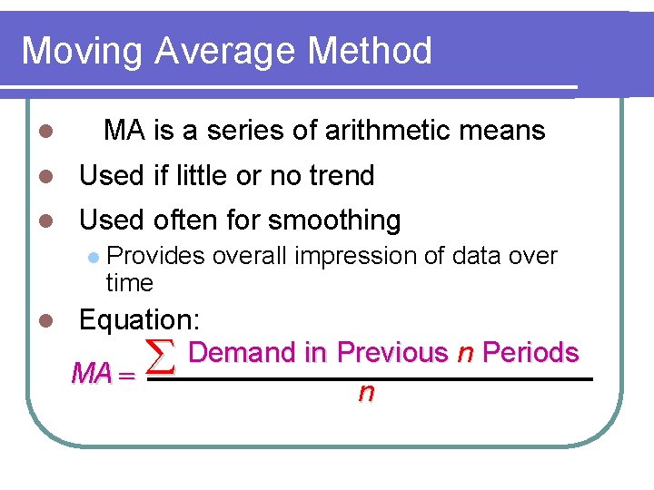
Moving Average Method MA is a series of arithmetic means l l Used if little or no trend l Used often for smoothing l l Provides overall impression of data over time Equation: Demand in Previous n Periods MA n

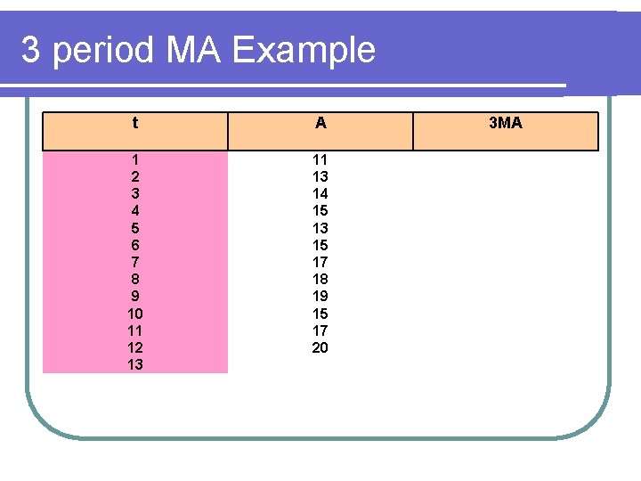
3 period MA Example t A 1 2 3 4 5 6 7 8 9 10 11 12 13 11 13 14 15 13 15 17 18 19 15 17 20 3 MA

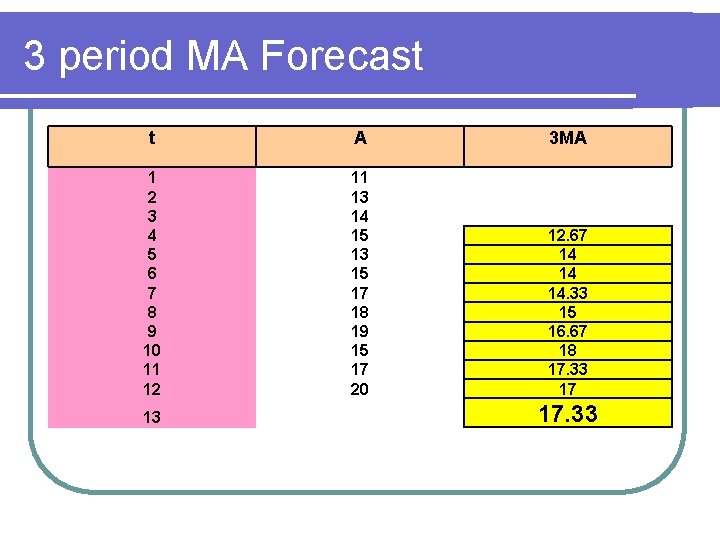
3 period MA Forecast t A 3 MA 1 2 3 4 5 6 7 8 9 10 11 12 11 13 14 15 13 15 17 18 19 15 17 20 12. 67 14 14 14. 33 15 16. 67 18 17. 33 17 13 17. 33

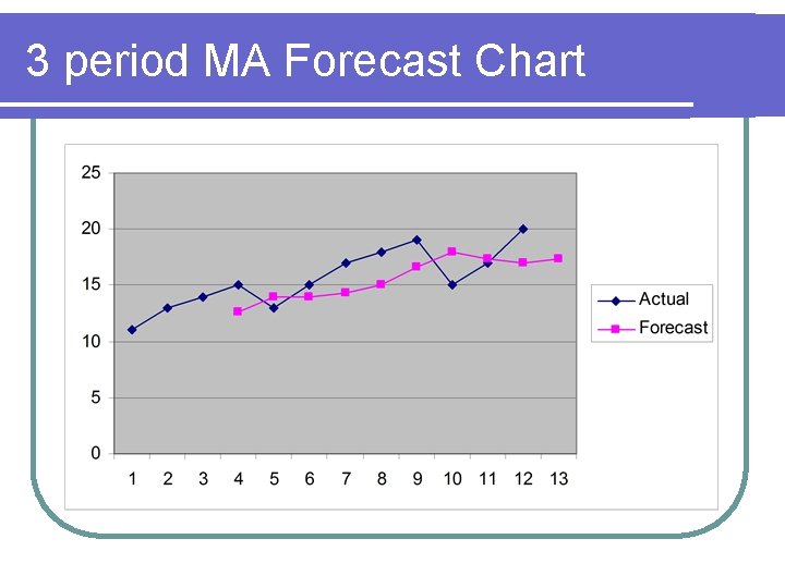
3 period MA Forecast Chart

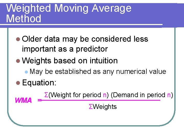
Weighted Moving Average Method l Older data may be considered less important as a predictor l Weights based on intuition l May be established as any numerical value l Equation: WMA = Σ(Weight for period n) (Demand in period n) ΣWeights

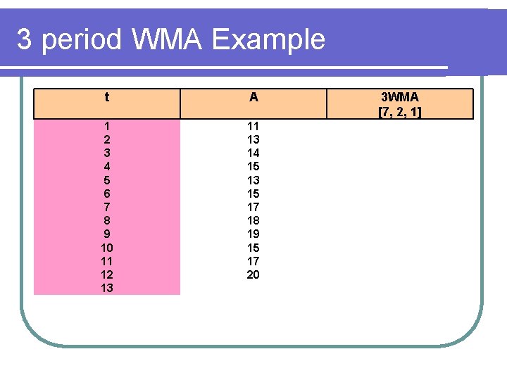
3 period WMA Example t A 1 2 3 4 5 6 7 8 9 10 11 12 13 11 13 14 15 13 15 17 18 19 15 17 20 3 WMA [7, 2, 1]

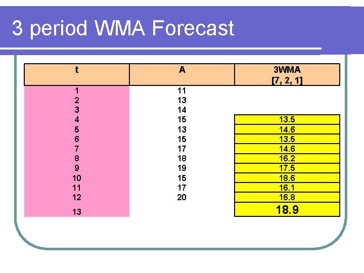
3 period WMA Forecast t A 1 2 3 4 5 6 7 8 9 10 11 12 11 13 14 15 13 15 17 18 19 15 17 20 13 3 WMA [7, 2, 1] 13. 5 14. 6 16. 2 17. 5 18. 6 16. 1 16. 8 18. 9

3 period WMA Forecast Chart

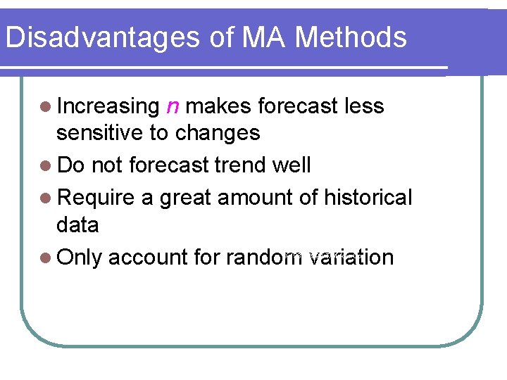
Disadvantages of MA Methods l Increasing n makes forecast less sensitive to changes l Do not forecast trend well l Require a great amount of historical data l Only account for random variation © 1984 -1994 T/Maker Co.

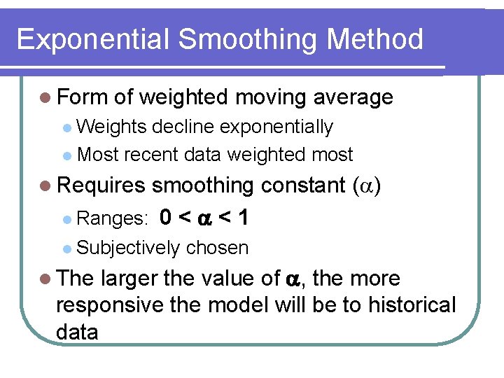
Exponential Smoothing Method l Form of weighted moving average l Weights decline exponentially l Most recent data weighted most l Requires smoothing constant ( ) l Ranges: 0 < < 1 l Subjectively chosen larger the value of , the more responsive the model will be to historical data l The

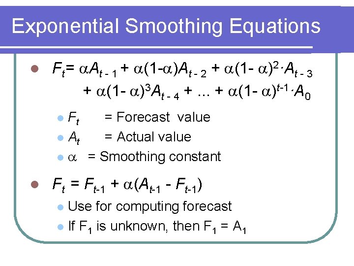
Exponential Smoothing Equations l Ft = At - 1 + (1 - )At - 2 + (1 - )2·At - 3 + (1 - )3 At - 4 +. . . + (1 - )t-1·A 0 Ft = Forecast value l At = Actual value l = Smoothing constant l l Ft = Ft-1 + (At-1 - Ft-1) Use for computing forecast l If F 1 is unknown, then F 1 = A 1 l

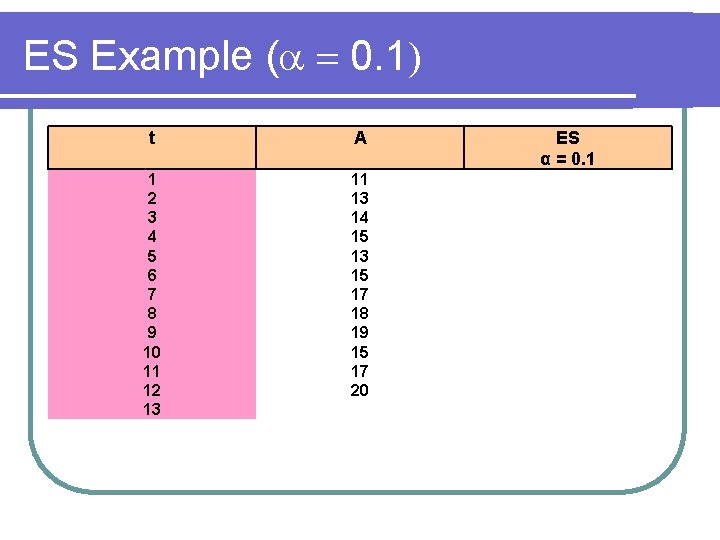
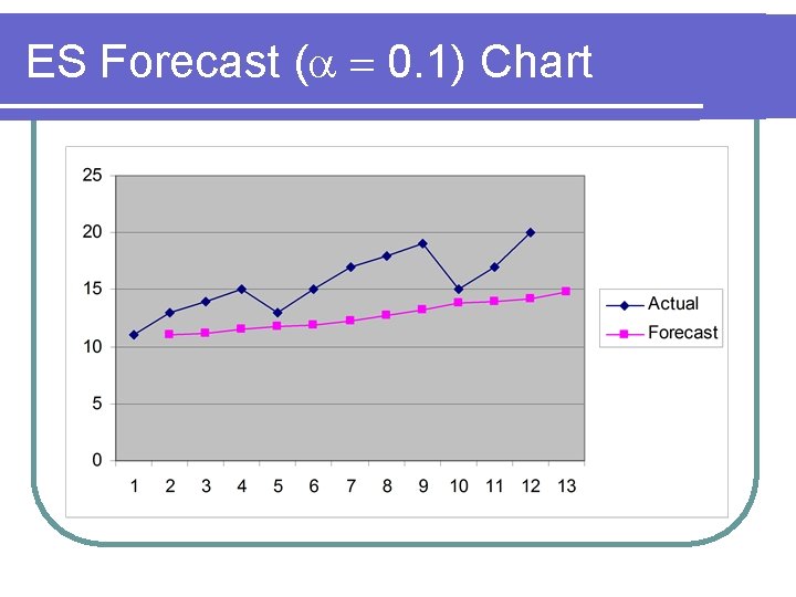
ES Example ( 0. 1) t A 1 2 3 4 5 6 7 8 9 10 11 12 13 11 13 14 15 13 15 17 18 19 15 17 20 ES α = 0. 1

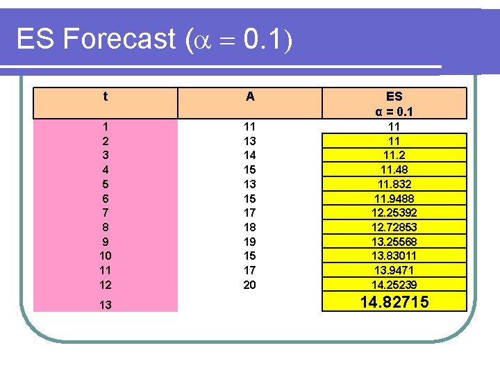
ES Forecast ( 0. 1) t A ES α = 0. 1 1 2 3 4 5 6 7 8 9 10 11 12 11 13 14 15 13 15 17 18 19 15 17 20 11 11 11. 2 11. 48 11. 832 11. 9488 12. 25392 12. 72853 13. 25568 13. 83011 13. 9471 14. 25239 13 14. 82715

ES Forecast ( 0. 1) Chart

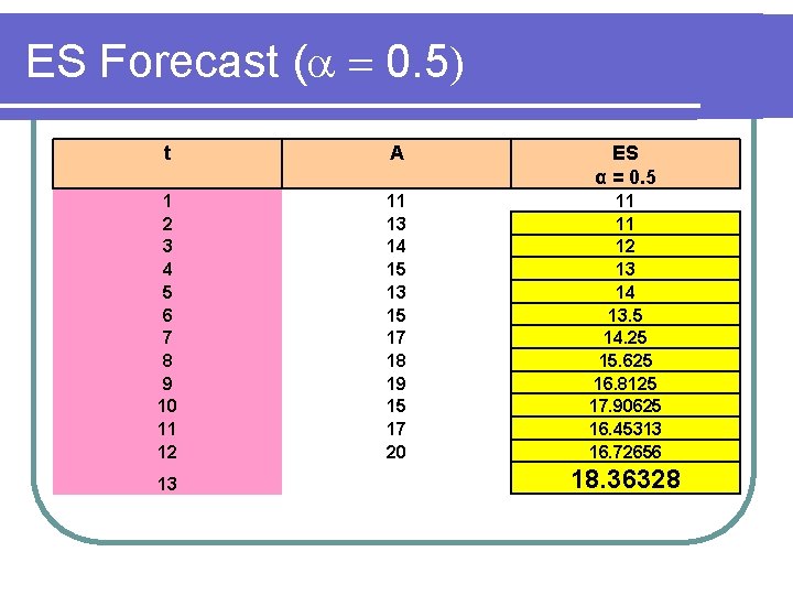
ES Example ( 0. 5) t A 1 2 3 4 5 6 7 8 9 10 11 12 13 11 13 14 15 13 15 17 18 19 15 17 20 ES α = 0. 5

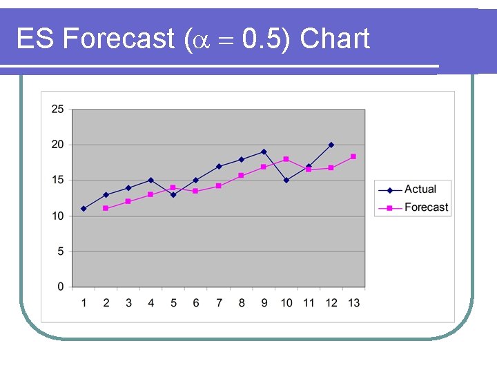
ES Forecast ( 0. 5) t A ES α = 0. 5 1 2 3 4 5 6 7 8 9 10 11 12 11 13 14 15 13 15 17 18 19 15 17 20 11 11 12 13 14 13. 5 14. 25 15. 625 16. 8125 17. 90625 16. 45313 16. 72656 13 18. 36328

ES Forecast ( 0. 5) Chart

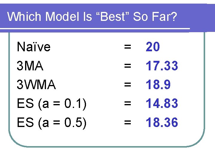
Which Model Is “Best” So Far? Naïve 3 MA 3 WMA ES (a = 0. 1) ES (a = 0. 5) = = = 20 17. 33 18. 9 14. 83 18. 36

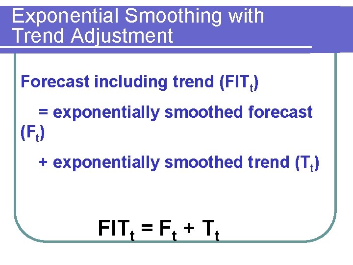
Exponential Smoothing with Trend Adjustment Forecast including trend (FITt) = exponentially smoothed forecast (Ft) + exponentially smoothed trend (Tt) FITt = Ft + Tt

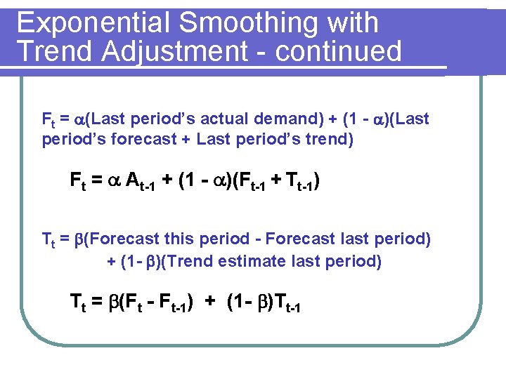
Exponential Smoothing with Trend Adjustment - continued Ft = (Last period’s actual demand) + (1 - )(Last period’s forecast + Last period’s trend) Ft = At-1 + (1 - )(Ft-1 + Tt-1) Tt = (Forecast this period - Forecast last period) + (1 - )(Trend estimate last period) Tt = (Ft - Ft-1) + (1 - )Tt-1

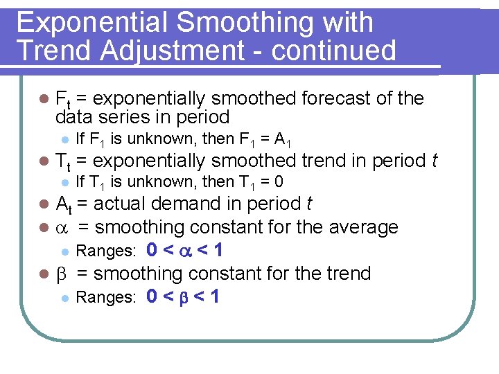
Exponential Smoothing with Trend Adjustment - continued l Ft = exponentially smoothed forecast of the data series in period l l If F 1 is unknown, then F 1 = A 1 Tt = exponentially smoothed trend in period t l If T 1 is unknown, then T 1 = 0 At = actual demand in period t = smoothing constant for the average l Ranges: 0 < < 1 l = smoothing constant for the trend l Ranges: 0 < < 1 l l

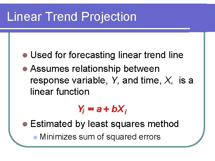
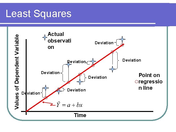
Linear Trend Projection l Used forecasting linear trend line l Assumes relationship between response variable, Y, and time, X, is a linear function Yi = a + b. X i l Estimated l by least squares method Minimizes sum of squared errors

Values of Dependent Variable Least Squares Actual observati on Deviation Deviation Time Point on regressio n line

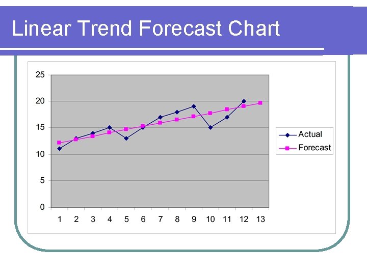
Linear Trend Forecast Chart

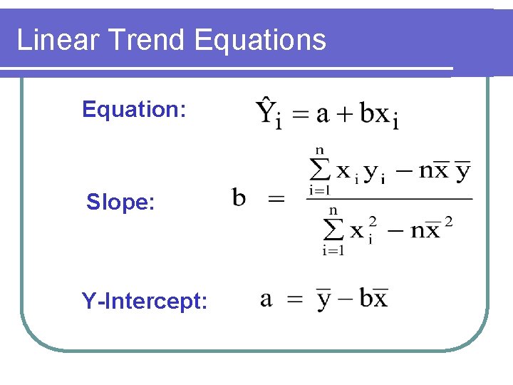
Linear Trend Equations Equation: Slope: Y-Intercept:

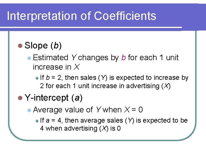
Interpretation of Coefficients l Slope (b) l Estimated Y changes by b for each 1 unit increase in X l If b = 2, then sales (Y) is expected to increase by 2 for each 1 unit increase in advertising (X) l Y-intercept l Average l If (a) value of Y when X = 0 a = 4, then average sales (Y) is expected to be 4 when advertising (X) is 0

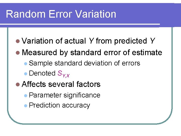
Random Error Variation l Variation of actual Y from predicted Y l Measured by standard error of estimate l Sample standard deviation of errors l Denoted SY, X l Affects several factors l Parameter significance l Prediction accuracy

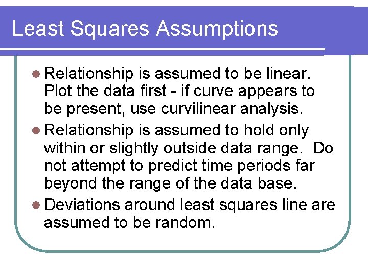
Least Squares Assumptions l Relationship is assumed to be linear. Plot the data first - if curve appears to be present, use curvilinear analysis. l Relationship is assumed to hold only within or slightly outside data range. Do not attempt to predict time periods far beyond the range of the data base. l Deviations around least squares line are assumed to be random.

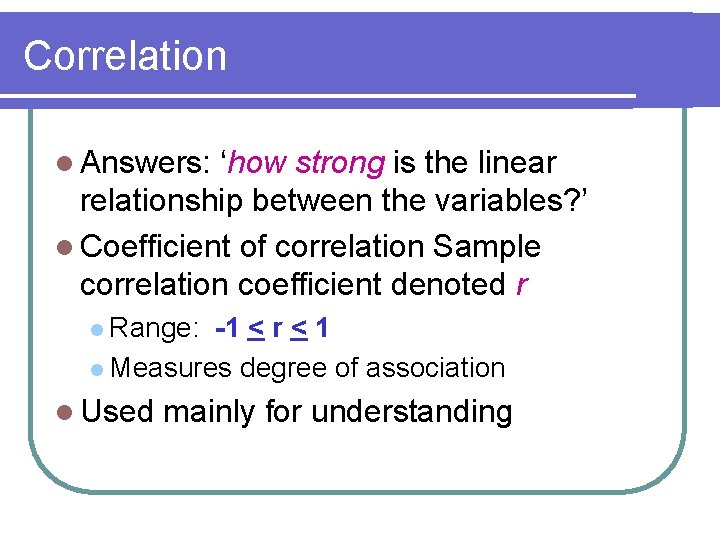
Correlation l Answers: ‘how strong is the linear relationship between the variables? ’ l Coefficient of correlation Sample correlation coefficient denoted r l Range: -1 < r < 1 l Measures degree of association l Used mainly for understanding

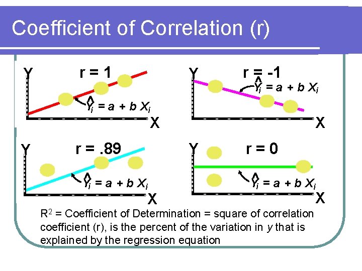
Coefficient of Correlation (r) Y r=1 Y ^i = a + b Xi Y r = -1 ^i = a + b Xi Y X Y r =. 89 ^i = a + b Xi Y X r=0 ^i = a + b Xi Y R 2 = Coefficient of Determination = square of correlation coefficient (r), is the percent of the variation in y that is explained by the regression equation X

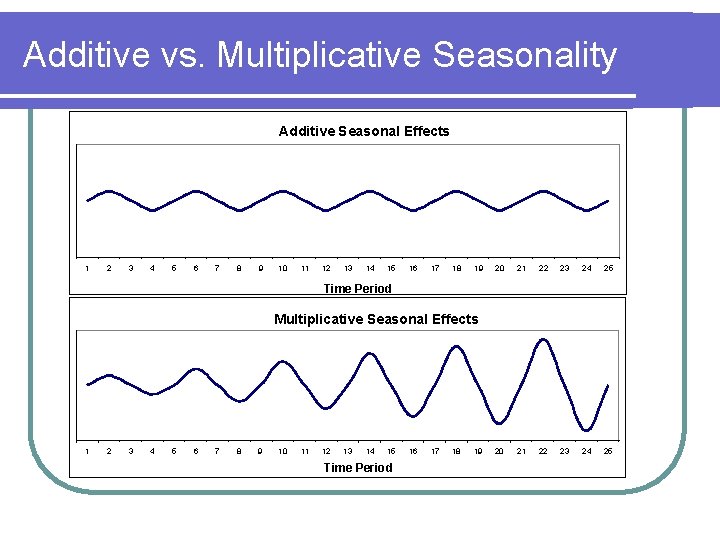
Additive vs. Multiplicative Seasonality Additive Seasonal Effects 1 2 3 4 5 6 7 8 9 10 11 12 13 14 15 16 17 18 19 20 21 22 23 24 25 Time Period Multiplicative Seasonal Effects 1 2 3 4 5 6 7 8 9 10 11 12 13 14 15 Time Period 16 17 18 19

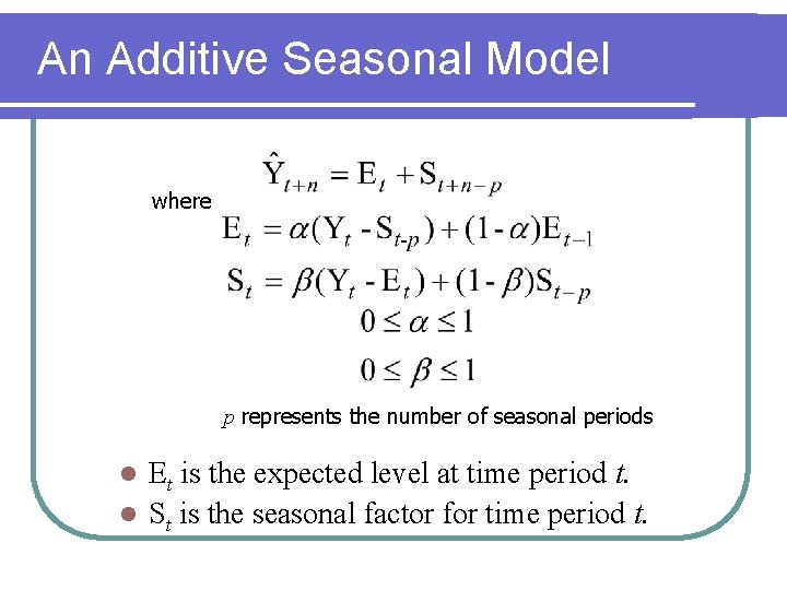
An Additive Seasonal Model where p represents the number of seasonal periods Et is the expected level at time period t. l St is the seasonal factor for time period t. l

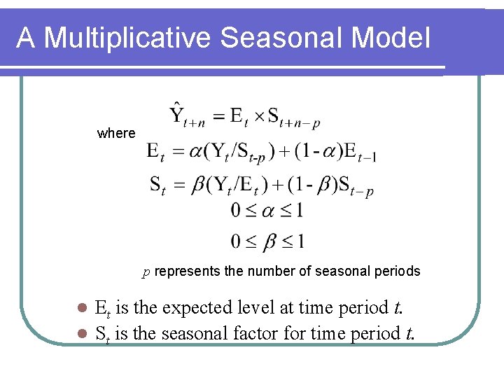
A Multiplicative Seasonal Model where p represents the number of seasonal periods Et is the expected level at time period t. l St is the seasonal factor for time period t. l

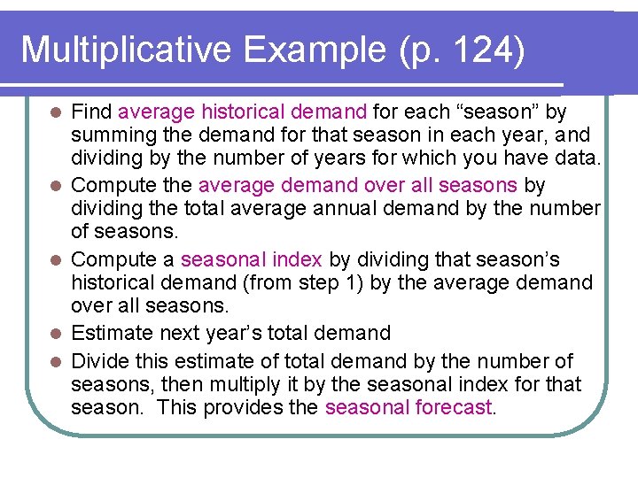
Multiplicative Example (p. 124) l l l Find average historical demand for each “season” by summing the demand for that season in each year, and dividing by the number of years for which you have data. Compute the average demand over all seasons by dividing the total average annual demand by the number of seasons. Compute a seasonal index by dividing that season’s historical demand (from step 1) by the average demand over all seasons. Estimate next year’s total demand Divide this estimate of total demand by the number of seasons, then multiply it by the seasonal index for that season. This provides the seasonal forecast.

Seasonal Example (p. 124) t Jan Feb Mar Apr May Jun Jul Aug Sep Oct Nov Dec Demand 2003 2004 2005 80 85 105 70 85 85 80 93 82 90 95 113 125 131 110 115 120 102 113 88 102 110 85 90 95 77 78 85 75 82 83 82 78 80 Average Monthly Demand Seasonal 2003 - 2005 Overall Index 90 94 0. 957 80 94 0. 851 85 94 0. 904 100 94 1. 064 123 94 1. 309 115 94 1. 223 105 94 1. 117 100 94 1. 064 90 94 0. 957 80 94 0. 851 2006 Forecast ? ? ?

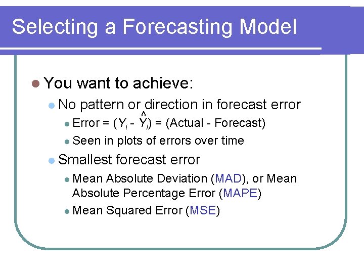
Selecting a Forecasting Model l You l No want to achieve: pattern or direction in forecast error l Error ^ = (Yi - Yi) = (Actual - Forecast) l Seen in plots of errors over time l Smallest l Mean forecast error Absolute Deviation (MAD), or Mean Absolute Percentage Error (MAPE) l Mean Squared Error (MSE)

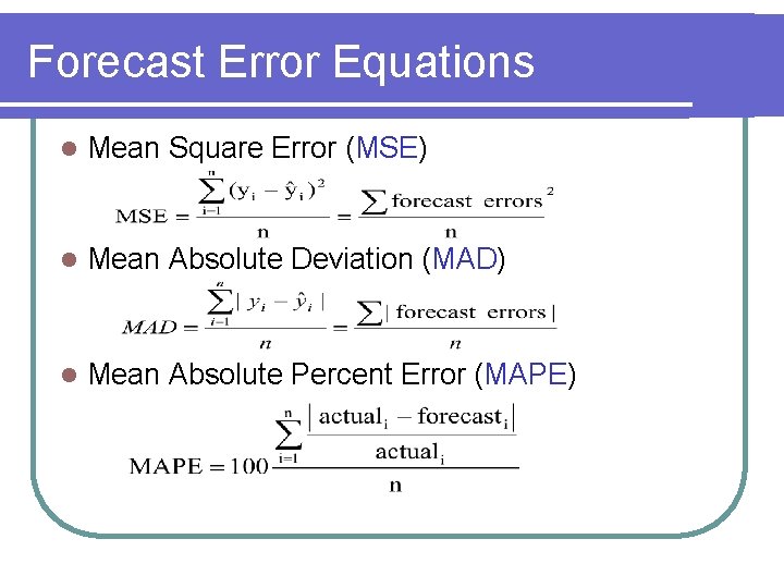
Forecast Error Equations l Mean Square Error (MSE) l Mean Absolute Deviation (MAD) l Mean Absolute Percent Error (MAPE)

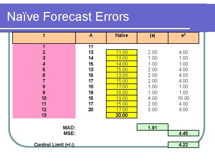
Naïve Forecast Errors t A 1 2 3 4 5 6 7 8 9 10 11 12 13 11 13 14 15 13 15 17 18 19 15 17 20 MAD: MSE: Control Limit (+/-): Naïve |e| e 2 11. 00 13. 00 14. 00 15. 00 13. 00 15. 00 17. 00 18. 00 19. 00 15. 00 17. 00 20. 00 2. 00 1. 00 4. 00 2. 00 3. 00 4. 00 16. 00 4. 00 9. 00 1. 91 4. 45 4. 22

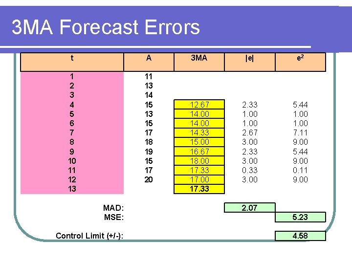
3 MA Forecast Errors t A 1 2 3 4 5 6 7 8 9 10 11 12 13 11 13 14 15 13 15 17 18 19 15 17 20 MAD: MSE: Control Limit (+/-): 3 MA |e| e 2 12. 67 14. 00 14. 33 15. 00 16. 67 18. 00 17. 33 17. 00 17. 33 2. 33 1. 00 2. 67 3. 00 2. 33 3. 00 0. 33 3. 00 5. 44 1. 00 7. 11 9. 00 5. 44 9. 00 0. 11 9. 00 2. 07 5. 23 4. 58

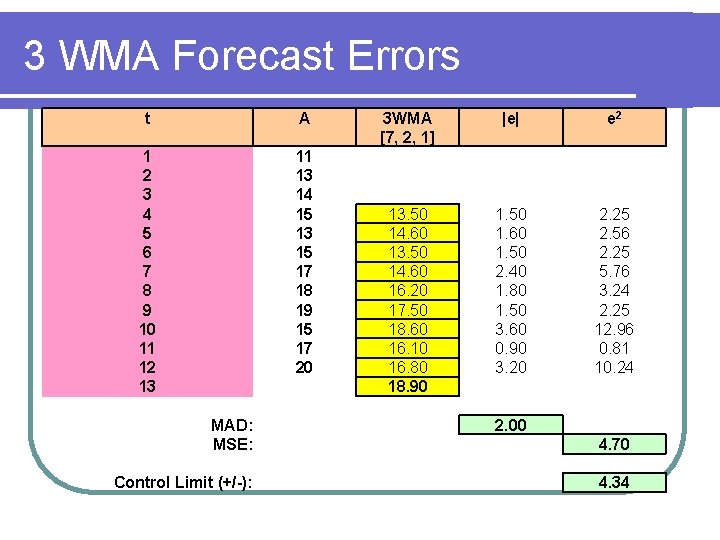
3 WMA Forecast Errors t A 1 2 3 4 5 6 7 8 9 10 11 12 13 11 13 14 15 13 15 17 18 19 15 17 20 MAD: MSE: Control Limit (+/-): 3 WMA [7, 2, 1] |e| e 2 13. 50 14. 60 16. 20 17. 50 18. 60 16. 10 16. 80 18. 90 1. 50 1. 60 1. 50 2. 40 1. 80 1. 50 3. 60 0. 90 3. 20 2. 25 2. 56 2. 25 5. 76 3. 24 2. 25 12. 96 0. 81 10. 24 2. 00 4. 70 4. 34

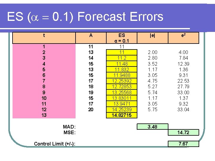
ES ( 0. 1) Forecast Errors t A 1 2 3 4 5 6 7 8 9 10 11 12 13 11 13 14 15 13 15 17 18 19 15 17 20 MAD: MSE: Control Limit (+/-): ES α = 0. 1 11 11 11. 2 11. 48 11. 832 11. 9488 12. 25392 12. 72853 13. 25568 13. 83011 13. 9471 14. 25239 14. 82715 |e| e 2 2. 00 2. 80 3. 52 1. 17 3. 05 4. 75 5. 27 5. 74 1. 17 3. 05 5. 75 4. 00 7. 84 12. 39 1. 36 9. 31 22. 53 27. 79 33. 00 1. 37 9. 32 33. 04 3. 48 14. 72 7. 67

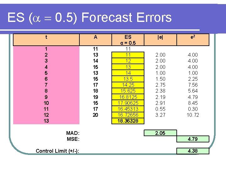
ES ( 0. 5) Forecast Errors t A 1 2 3 4 5 6 7 8 9 10 11 12 13 11 13 14 15 13 15 17 18 19 15 17 20 MAD: MSE: Control Limit (+/-): ES α = 0. 5 11 11 12 13 14 13. 5 14. 25 15. 625 16. 8125 17. 90625 16. 45313 16. 72656 18. 36328 |e| e 2 2. 00 1. 50 2. 75 2. 38 2. 19 2. 91 0. 55 3. 27 4. 00 1. 00 2. 25 7. 56 5. 64 4. 79 8. 45 0. 30 10. 72 2. 05 4. 79 4. 38

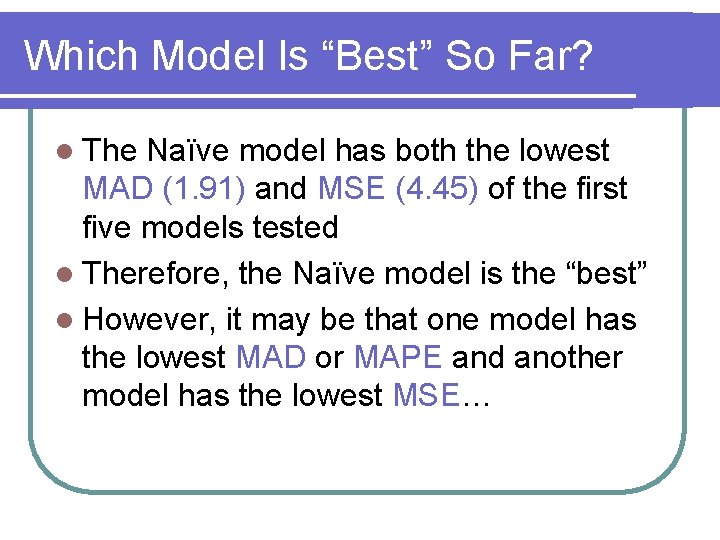
Which Model Is “Best” So Far? l The Naïve model has both the lowest MAD (1. 91) and MSE (4. 45) of the first five models tested l Therefore, the Naïve model is the “best” l However, it may be that one model has the lowest MAD or MAPE and another model has the lowest MSE…

So Which Model Do You Choose? l If you only require the forecast with the smallest average deviation, choose the model with the smallest MAD or MAPE l However, if you have a low tolerance for large deviations choose the model with the smallest MSE

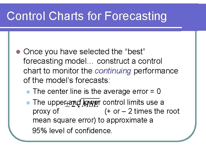
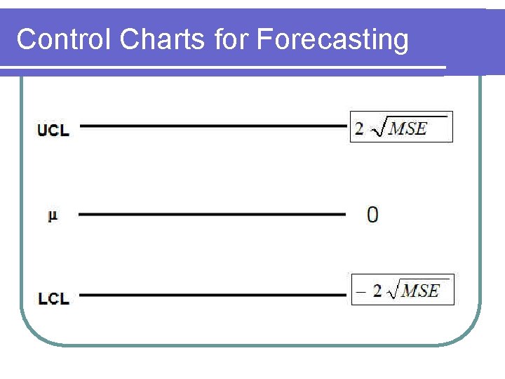
Control Charts for Forecasting l Once you have selected the “best” forecasting model… construct a control chart to monitor the continuing performance of the model’s forecasts: The center line is the average error = 0 l The upper and lower control limits use a proxy of (+ or – 2 times the root mean square error) to approximate a 95% level of confidence. l

Control Charts for Forecasting

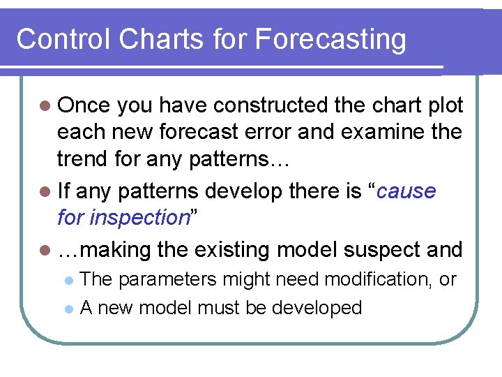
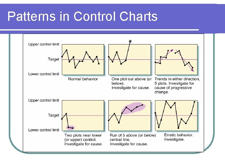
Control Charts for Forecasting l Once you have constructed the chart plot each new forecast error and examine the trend for any patterns… l If any patterns develop there is “cause for inspection” l …making the existing model suspect and The parameters might need modification, or l A new model must be developed l

Patterns in Control Charts

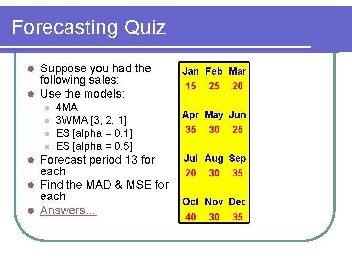
Forecasting Quiz Suppose you had the following sales: l Use the models: l l l 4 MA 3 WMA [3, 2, 1] ES [alpha = 0. 5] Forecast period 13 for each l Find the MAD & MSE for each l Answers… l Jan Feb Mar 15 25 20 Apr May Jun 35 30 25 Jul Aug Sep 20 30 35 Oct Nov Dec 40 30 35