Forecasting Models2 MULTIPLICATIVE DECOMPOSITION SAWYER PIANO HOUSE EXAMPLE

Forecasting Models-2

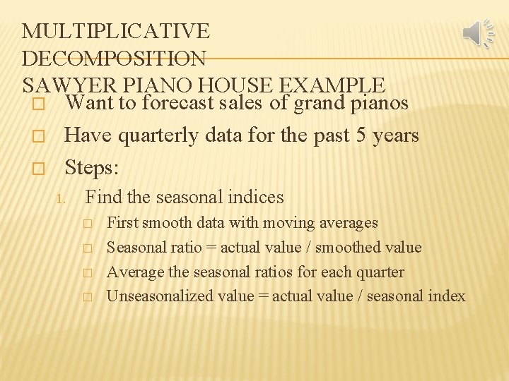
MULTIPLICATIVE DECOMPOSITION SAWYER PIANO HOUSE EXAMPLE � Want to forecast sales of grand pianos � Have quarterly data for the past 5 years � Steps: 1. Find the seasonal indices � � First smooth data with moving averages Seasonal ratio = actual value / smoothed value Average the seasonal ratios for each quarter Unseasonalized value = actual value / seasonal index

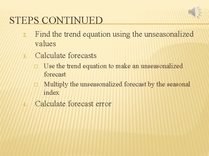
STEPS CONTINUED 2. 3. Find the trend equation using the unseasonalized values Calculate forecasts � � 4. Use the trend equation to make an unseasonalized forecast Multiply the unseasonalized forecast by the seasonal index Calculate forecast error

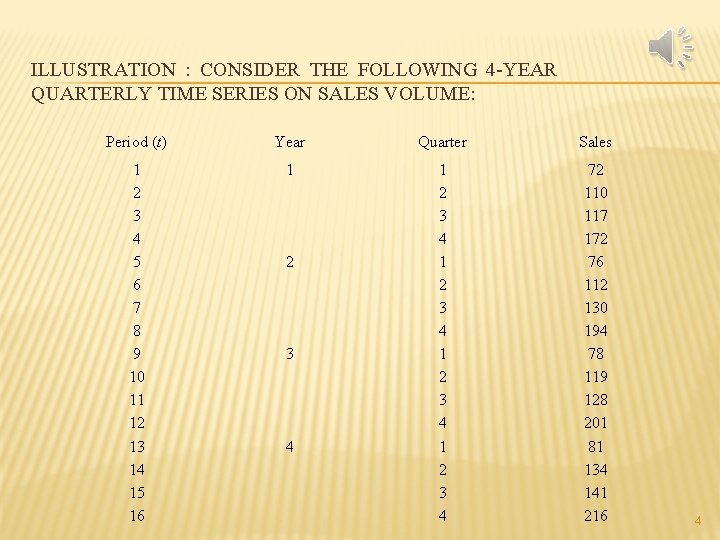
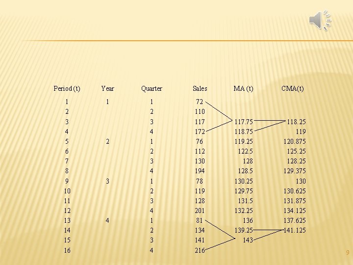
ILLUSTRATION : CONSIDER THE FOLLOWING 4 -YEAR QUARTERLY TIME SERIES ON SALES VOLUME: Period (t) Year Quarter Sales 1 2 3 4 5 6 7 8 9 10 11 12 13 14 15 16 1 1 2 3 4 72 110 117 172 76 112 130 194 78 119 128 201 81 134 141 216 2 3 4 4

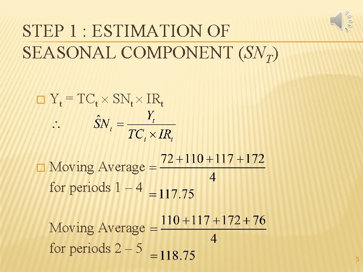
STEP 1 : ESTIMATION OF SEASONAL COMPONENT (SNT) � � Yt = TCt SNt IRt Moving Average for periods 1 – 4 Moving Average for periods 2 – 5 5

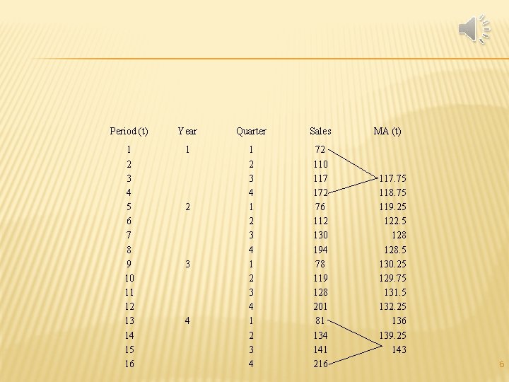
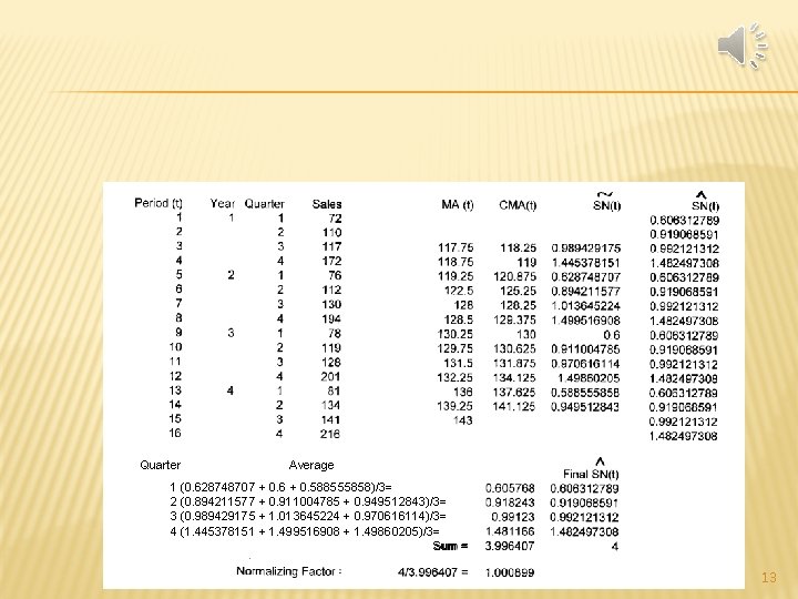
Period (t) Year Quarter Sales 1 2 3 4 5 6 7 8 9 10 11 12 13 14 15 16 1 1 2 3 4 72 110 117 172 76 112 130 194 78 119 128 201 81 134 141 216 2 3 4 MA (t) 117. 75 118. 75 119. 25 122. 5 128. 5 130. 25 129. 75 131. 5 132. 25 136 139. 25 143 6

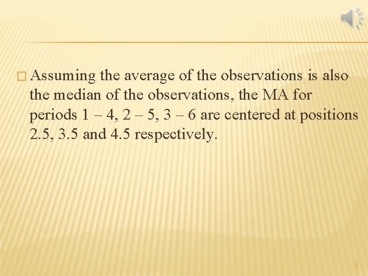
� Assuming the average of the observations is also the median of the observations, the MA for periods 1 – 4, 2 – 5, 3 – 6 are centered at positions 2. 5, 3. 5 and 4. 5 respectively. 7

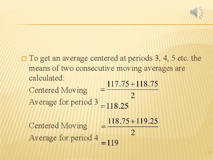
� To get an average centered at periods 3, 4, 5 etc. the means of two consecutive moving averages are calculated: Centered Moving Average for period 3 Centered Moving Average for period 4 8

Period (t) Year Quarter Sales 1 2 3 4 5 6 7 8 9 10 11 12 13 14 15 16 1 1 2 3 4 72 110 117 172 76 112 130 194 78 119 128 201 81 134 141 216 2 3 4 MA (t) CMA(t) 117. 75 118. 75 119. 25 122. 5 128. 5 130. 25 129. 75 131. 5 132. 25 136 139. 25 143 118. 25 119 120. 875 125. 25 128. 25 129. 375 130. 625 131. 875 134. 125 137. 625 141. 125 9

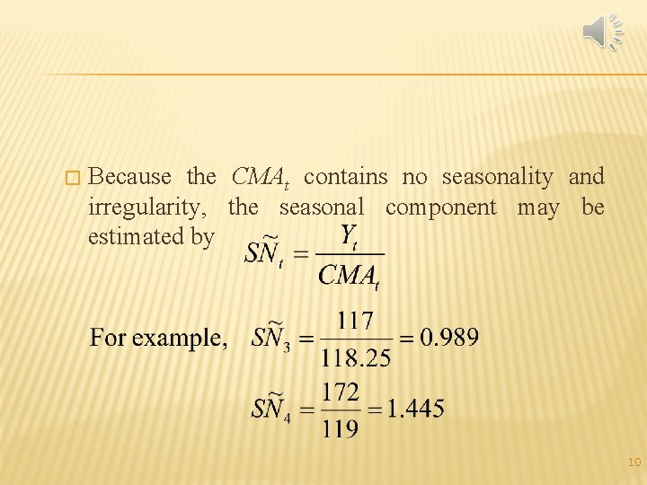
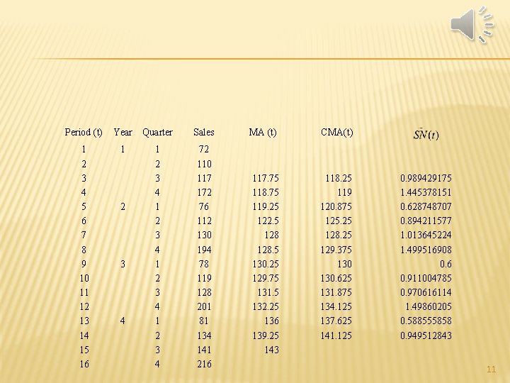
� Because the CMAt contains no seasonality and irregularity, the seasonal component may be estimated by 10

Period (t) Year Quarter Sales 1 2 3 4 5 6 7 8 9 10 11 12 13 14 15 16 1 1 2 3 4 72 110 117 172 76 112 130 194 78 119 128 201 81 134 141 216 2 3 4 MA (t) CMA(t) 117. 75 118. 75 119. 25 122. 5 128. 5 130. 25 129. 75 131. 5 132. 25 136 139. 25 143 118. 25 119 120. 875 125. 25 128. 25 129. 375 130. 625 131. 875 134. 125 137. 625 141. 125 0. 989429175 1. 445378151 0. 628748707 0. 894211577 1. 013645224 1. 499516908 0. 6 0. 911004785 0. 970616114 1. 49860205 0. 588555858 0. 949512843 11

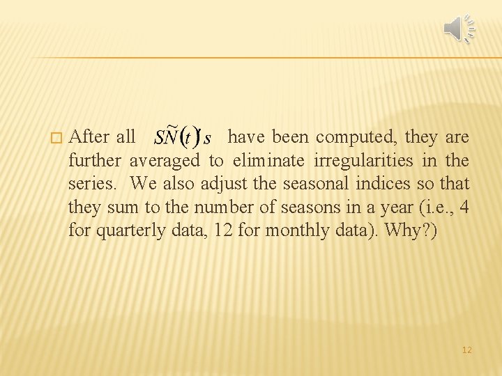
� After all have been computed, they are further averaged to eliminate irregularities in the series. We also adjust the seasonal indices so that they sum to the number of seasons in a year (i. e. , 4 for quarterly data, 12 for monthly data). Why? ) 12

Quarter Average 1 (0. 628748707 + 0. 6 + 0. 588555858)/3= 2 (0. 894211577 + 0. 911004785 + 0. 949512843)/3= 3 (0. 989429175 + 1. 013645224 + 0. 970616114)/3= 4 (1. 445378151 + 1. 499516908 + 1. 49860205)/3= Sum = 13

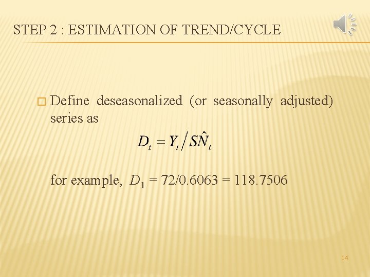
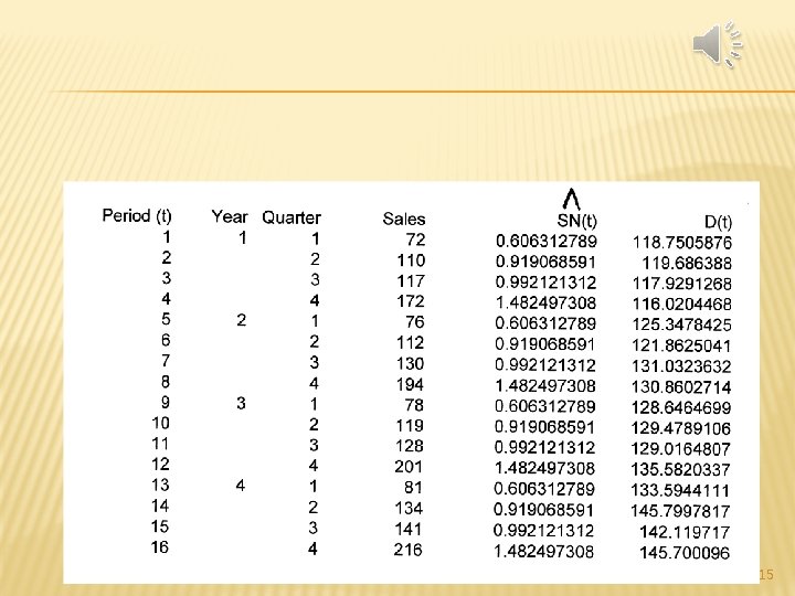
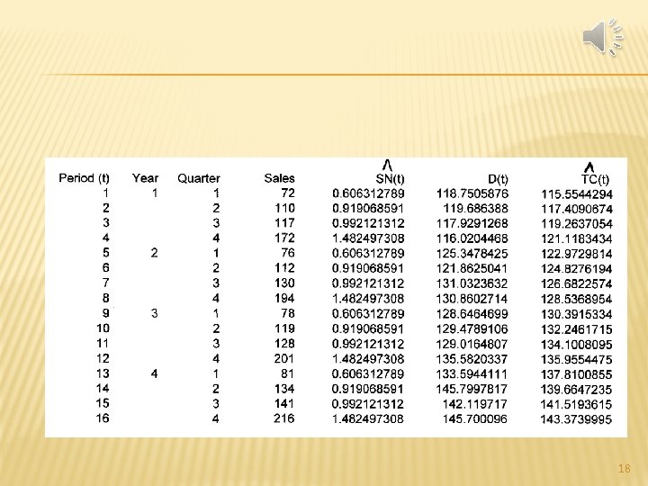
STEP 2 : ESTIMATION OF TREND/CYCLE � Define deseasonalized (or seasonally adjusted) series as for example, D 1 = 72/0. 6063 = 118. 7506 14

15

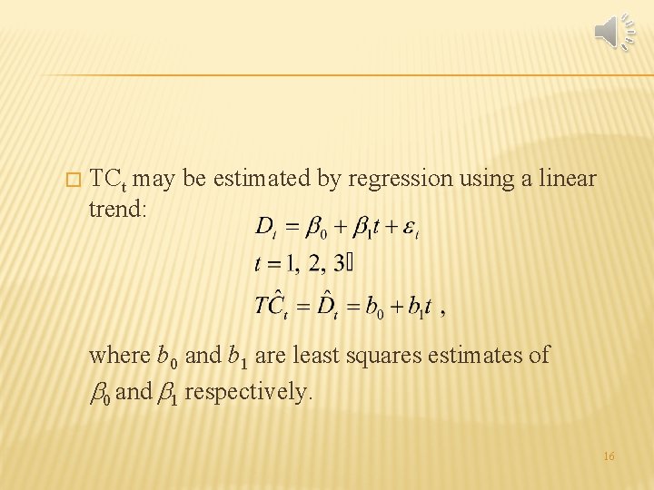
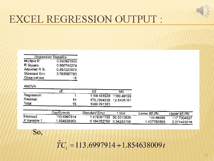
� TCt may be estimated by regression using a linear trend: where b 0 and b 1 are least squares estimates of 0 and 1 respectively. 16

EXCEL REGRESSION OUTPUT : 17

18

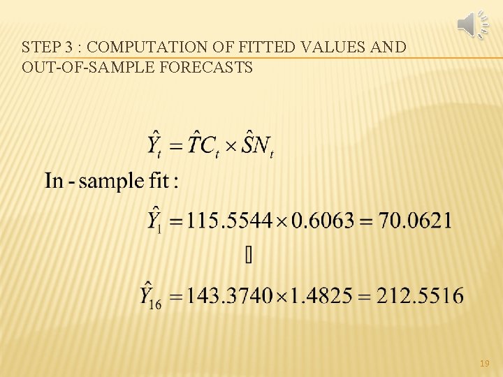
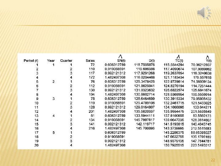
STEP 3 : COMPUTATION OF FITTED VALUES AND OUT-OF-SAMPLE FORECASTS 19

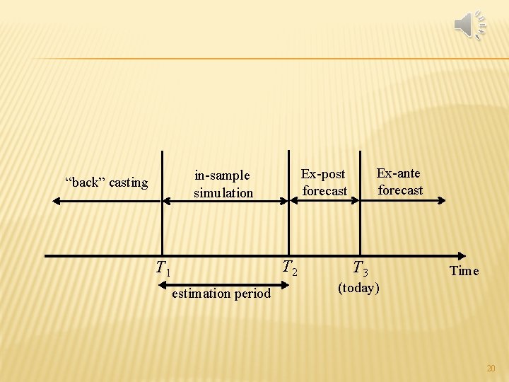
“back” casting T 2 T 1 estimation period Ex-ante forecast Ex-post forecast in-sample simulation T 3 Time (today) 20

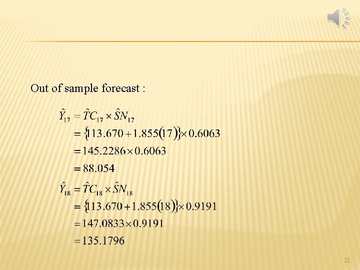
Out of sample forecast : 21

22