Forecasting Chapter 13 To Accompany Krajewski Ritzman Operations




- Slides: 83

Forecasting Chapter 13 To Accompany Krajewski & Ritzman Operations Management: Strategy and Analysis, Seventh Edition © 2004 Prentice Hall, Inc. All rights reserved.

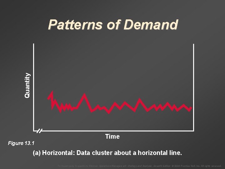
Quantity Patterns of Demand Time Figure 13. 1 (a) Horizontal: Data cluster about a horizontal line. To Accompany Krajewski & Ritzman Operations Management: Strategy and Analysis, Seventh Edition © 2004 Prentice Hall, Inc. All rights reserved.

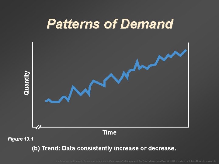
Quantity Patterns of Demand Time Figure 13. 1 (b) Trend: Data consistently increase or decrease. To Accompany Krajewski & Ritzman Operations Management: Strategy and Analysis, Seventh Edition © 2004 Prentice Hall, Inc. All rights reserved.

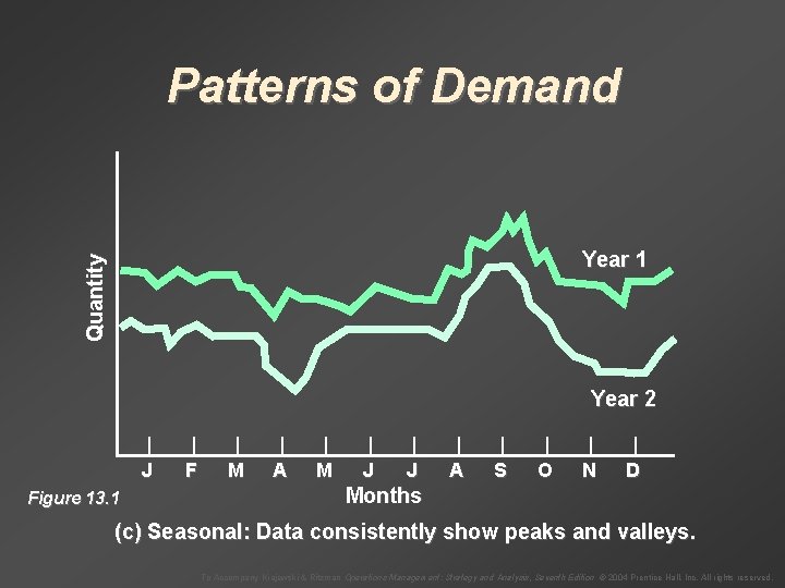
Patterns of Demand Quantity Year 1 Year 2 Figure 13. 1 | | | J F M A M J J A S O N D Months (c) Seasonal: Data consistently show peaks and valleys. To Accompany Krajewski & Ritzman Operations Management: Strategy and Analysis, Seventh Edition © 2004 Prentice Hall, Inc. All rights reserved.

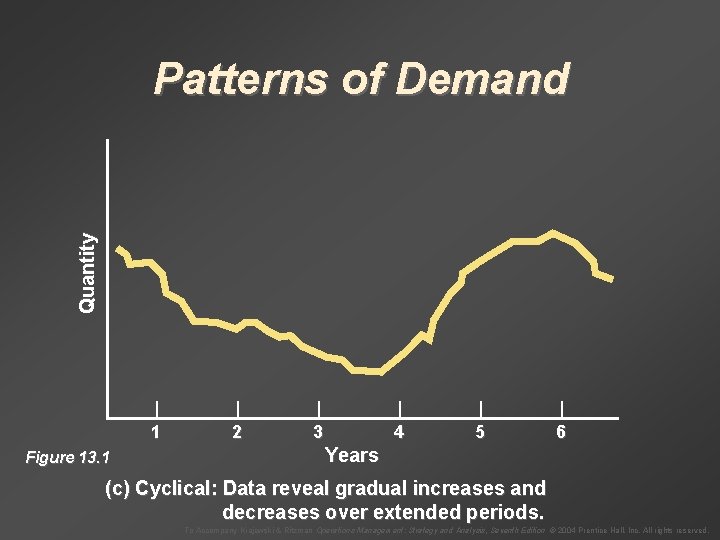
Quantity Patterns of Demand Figure 13. 1 | | | 1 2 3 4 5 6 Years (c) Cyclical: Data reveal gradual increases and decreases over extended periods. To Accompany Krajewski & Ritzman Operations Management: Strategy and Analysis, Seventh Edition © 2004 Prentice Hall, Inc. All rights reserved.

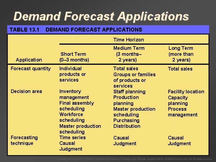
Demand Forecast Applications TABLE 13. 1 DEMAND FORECAST APPLICATIONS Time Horizon Application Short Term (0– 3 months) Forecast quantity Individual products or services Decision area Inventory management Final assembly scheduling Workforce scheduling Master production scheduling Time series Causal Judgment Forecasting technique Medium Term (3 months– 2 years) Long Term (more than 2 years) Total sales Groups or families of products or services Staff planning Production planning Master production scheduling Purchasing Distribution Total sales Causal Judgment Facility location Capacity planning Process management To Accompany Krajewski & Ritzman Operations Management: Strategy and Analysis, Seventh Edition © 2004 Prentice Hall, Inc. All rights reserved.

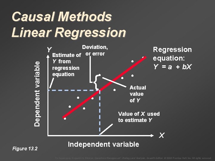
Causal Methods Linear Regression Dependent variable Y Deviation, Estimate of or error Y from regression equation { Regression equation: Y = a + b. X Actual value of Y Value of X used to estimate Y X Figure 13. 2 Independent variable To Accompany Krajewski & Ritzman Operations Management: Strategy and Analysis, Seventh Edition © 2004 Prentice Hall, Inc. All rights reserved.

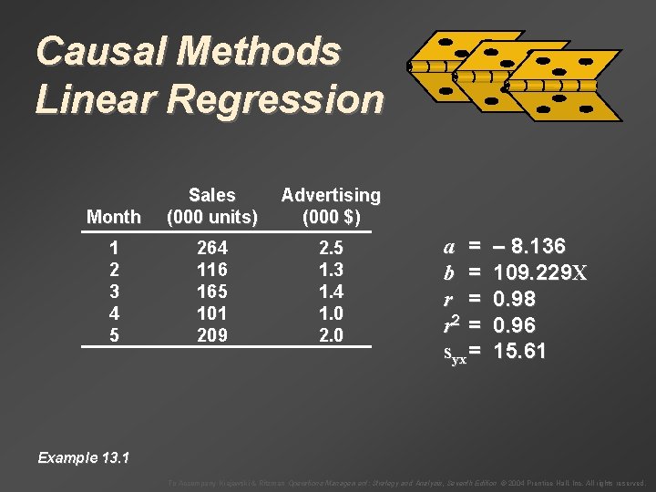
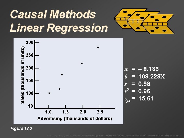
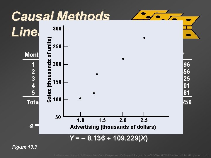
Causal Methods Linear Regression Month Sales (000 units) Advertising (000 $) 1 2 3 4 5 264 116 165 101 209 2. 5 1. 3 1. 4 1. 0 2. 0 a = b = r 2 = syx = – 8. 136 109. 229 X 0. 98 0. 96 15. 61 Example 13. 1 To Accompany Krajewski & Ritzman Operations Management: Strategy and Analysis, Seventh Edition © 2004 Prentice Hall, Inc. All rights reserved.

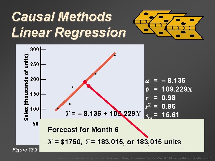
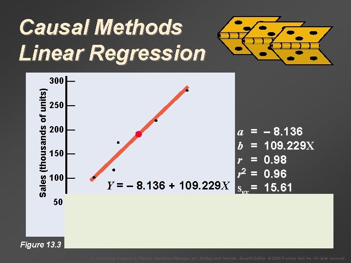
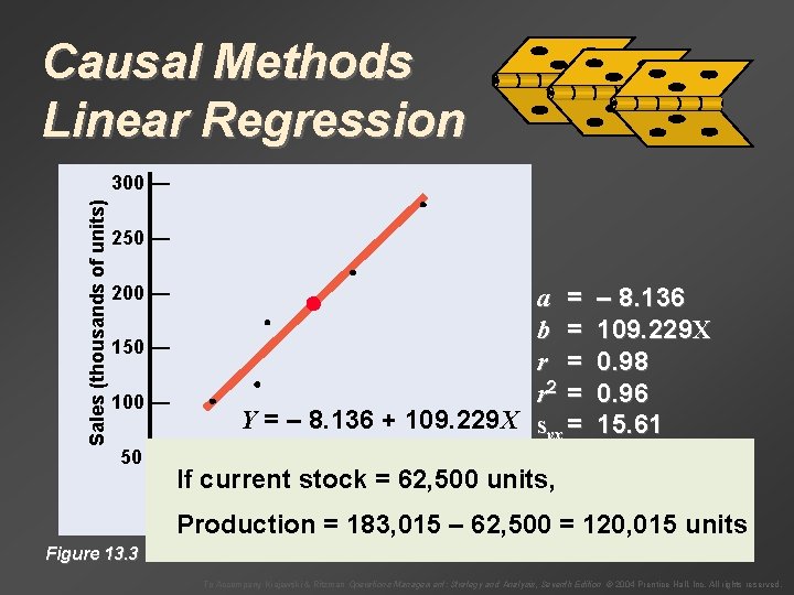
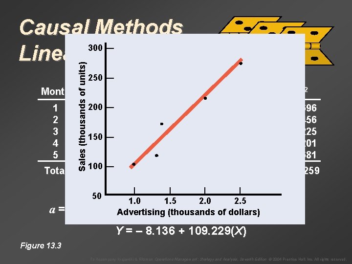
Causal Methods Linear Regression Sales (thousands of units) 300 — 250 — Month Sales (000 units) Advertising (000 $) 1 2 150 — 3 4 100 — 5 264 116 165 101 209 2. 5 1. 3 1. 4 1. 0 200 — 50 a = b = r 2 = syx = – 8. 136 109. 229 X 0. 98 0. 96 15. 61 | | 1. 0 1. 5 2. 0 2. 5 Advertising (thousands of dollars) Figure 13. 3 To Accompany Krajewski & Ritzman Operations Management: Strategy and Analysis, Seventh Edition © 2004 Prentice Hall, Inc. All rights reserved.

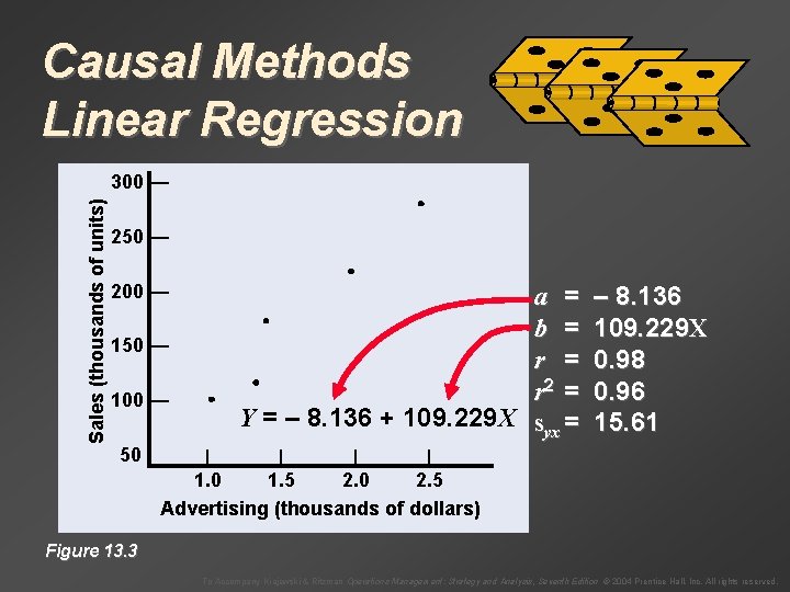
Causal Methods Linear Regression Sales (thousands of units) 300 — 250 — Month Sales (000 units) 1 2 150 — 3 4 100 — 5 264 116 165 101 209 Y= 200 — 50 Advertising (000 $) – 8. 136 2. 5 1. 3 1. 4 1. 0 +2. 0109. 229 X a = b = r 2 = syx = – 8. 136 109. 229 X 0. 98 0. 96 15. 61 | | 1. 0 1. 5 2. 0 2. 5 Advertising (thousands of dollars) Figure 13. 3 To Accompany Krajewski & Ritzman Operations Management: Strategy and Analysis, Seventh Edition © 2004 Prentice Hall, Inc. All rights reserved.

Causal Methods Linear Regression Sales (thousands of units) 300 — 250 — Month Sales (000 units) 1 2 150 — 3 4 100 — 5 264 116 165 101 209 Y= 200 — 50 Advertising (000 $) – 8. 136 2. 5 1. 3 1. 4 1. 0 +2. 0109. 229 X a = b = r 2 = syx = – 8. 136 109. 229 X 0. 98 0. 96 15. 61 | | 1. 0 1. 5 2. 0 2. 5 Advertising (thousands of dollars) Figure 13. 3 To Accompany Krajewski & Ritzman Operations Management: Strategy and Analysis, Seventh Edition © 2004 Prentice Hall, Inc. All rights reserved.

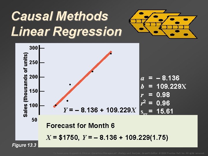
Causal Methods Linear Regression Sales (thousands of units) 300 — 250 — Month Sales (000 units) 1 2 150 — 3 4 100 — 5 264 116 165 101 209 Y= 200 — 50 Advertising (000 $) – 8. 136 2. 5 1. 3 1. 4 1. 0 +2. 0109. 229 X a = b = r 2 = syx = – 8. 136 109. 229 X 0. 98 0. 96 15. 61 | | Forecast 6 1. 0 1. 5 for Month 2. 0 2. 5 Advertising (thousands of dollars) X = $1750, Y = – 8. 136 + 109. 229(1. 75) Figure 13. 3 To Accompany Krajewski & Ritzman Operations Management: Strategy and Analysis, Seventh Edition © 2004 Prentice Hall, Inc. All rights reserved.

Causal Methods Linear Regression Sales (thousands of units) 300 — 250 — Month Sales (000 units) 1 2 150 — 3 4 100 — 5 264 116 165 101 209 Y= 200 — 50 Advertising (000 $) – 8. 136 2. 5 1. 3 1. 4 1. 0 +2. 0109. 229 X a = b = r 2 = syx = – 8. 136 109. 229 X 0. 98 0. 96 15. 61 | | Forecast 6 1. 0 1. 5 for Month 2. 0 2. 5 Advertising (thousands of dollars) X = $1750, Y = 183. 015, or 183, 015 units Figure 13. 3 To Accompany Krajewski & Ritzman Operations Management: Strategy and Analysis, Seventh Edition © 2004 Prentice Hall, Inc. All rights reserved.

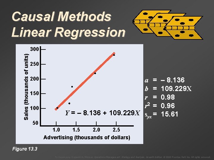
Causal Methods Linear Regression Sales (thousands of units) 300 — 250 — Month Sales (000 units) 1 2 150 — 3 4 100 — 5 264 116 165 101 209 Y= 200 — 50 Advertising (000 $) – 8. 136 2. 5 1. 3 1. 4 1. 0 +2. 0109. 229 X a = b = r 2 = syx = – 8. 136 109. 229 X 0. 98 0. 96 15. 61 | | 1. 0 1. 5 2. 0 2. 5 Advertising (thousands of dollars) Figure 13. 3 To Accompany Krajewski & Ritzman Operations Management: Strategy and Analysis, Seventh Edition © 2004 Prentice Hall, Inc. All rights reserved.

Causal Methods Linear Regression Sales (thousands of units) 300 — 250 — Month Sales (000 units) 1 2 150 — 3 4 100 — 5 264 116 165 101 209 Y= 200 — 50 Advertising (000 $) – 8. 136 2. 5 1. 3 1. 4 1. 0 +2. 0109. 229 X a = b = r 2 = syx = – 8. 136 109. 229 X 0. 98 0. 96 15. 61 | | If 1. 0 current units, 1. 5 stock 2. 0 = 62, 500 2. 5 Advertising (thousands of dollars) Production = 183, 015 – 62, 500 = 120, 015 units Figure 13. 3 To Accompany Krajewski & Ritzman Operations Management: Strategy and Analysis, Seventh Edition © 2004 Prentice Hall, Inc. All rights reserved.

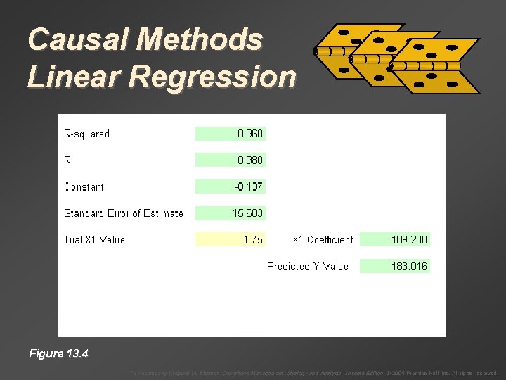
Causal Methods Linear Regression Figure 13. 4 To Accompany Krajewski & Ritzman Operations Management: Strategy and Analysis, Seventh Edition © 2004 Prentice Hall, Inc. All rights reserved.

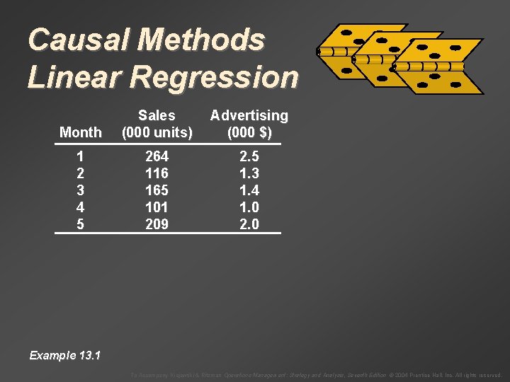
Causal Methods Linear Regression Month Sales (000 units) Advertising (000 $) 1 2 3 4 5 264 116 165 101 209 2. 5 1. 3 1. 4 1. 0 2. 0 Example 13. 1 To Accompany Krajewski & Ritzman Operations Management: Strategy and Analysis, Seventh Edition © 2004 Prentice Hall, Inc. All rights reserved.

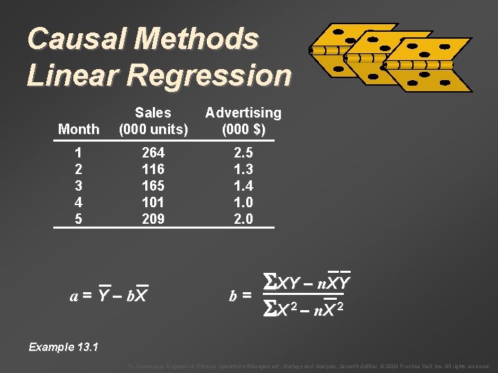
Causal Methods Linear Regression Month Sales (000 units) Advertising (000 $) 1 2 3 4 5 264 116 165 101 209 2. 5 1. 3 1. 4 1. 0 2. 0 a = Y – b. X b= XY – n. XY X 2 – n. X 2 Example 13. 1 To Accompany Krajewski & Ritzman Operations Management: Strategy and Analysis, Seventh Edition © 2004 Prentice Hall, Inc. All rights reserved.

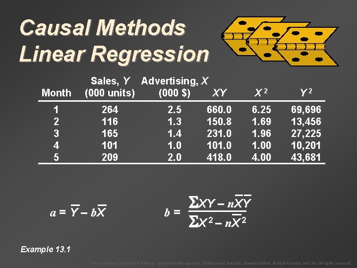
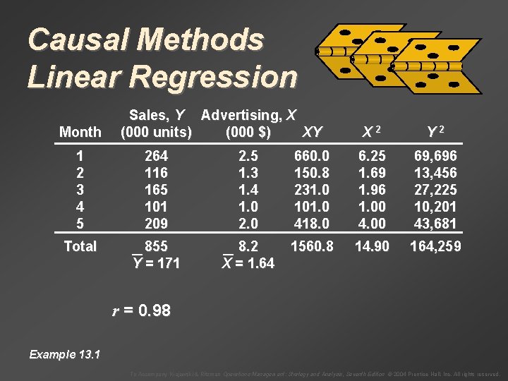
Causal Methods Linear Regression Month 1 2 3 4 5 Sales, Y Advertising, X (000 units) (000 $) XY 264 116 165 101 209 a = Y – b. X 2. 5 1. 3 1. 4 1. 0 2. 0 660. 0 150. 8 231. 0 101. 0 418. 0 b= XY – n. XY X 2 – n. X 2 Y 2 6. 25 1. 69 1. 96 1. 00 4. 00 69, 696 13, 456 27, 225 10, 201 43, 681 Example 13. 1 To Accompany Krajewski & Ritzman Operations Management: Strategy and Analysis, Seventh Edition © 2004 Prentice Hall, Inc. All rights reserved.

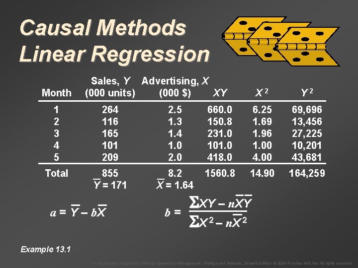
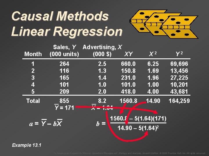
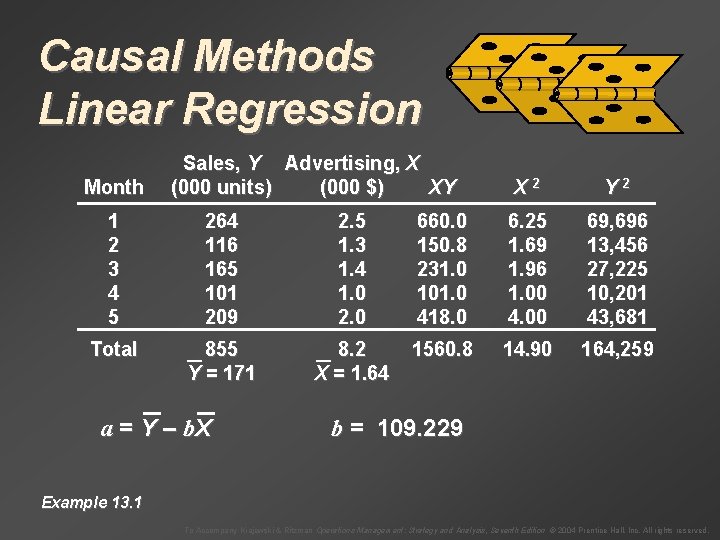
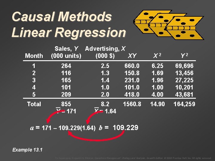
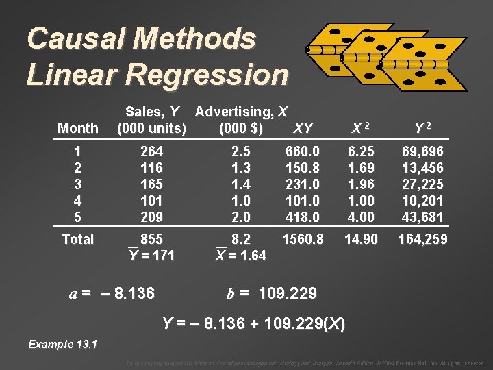
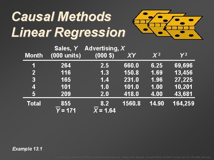
Causal Methods Linear Regression Month Sales, Y Advertising, X (000 units) (000 $) XY X 2 Y 2 1 2 3 4 5 264 116 165 101 209 2. 5 1. 3 1. 4 1. 0 2. 0 660. 0 150. 8 231. 0 101. 0 418. 0 6. 25 1. 69 1. 96 1. 00 4. 00 69, 696 13, 456 27, 225 10, 201 43, 681 Total 855 Y = 171 8. 2 X = 1. 64 1560. 8 14. 90 164, 259 a = Y – b. X b= XY – n. XY X 2 – n. X 2 Example 13. 1 To Accompany Krajewski & Ritzman Operations Management: Strategy and Analysis, Seventh Edition © 2004 Prentice Hall, Inc. All rights reserved.

Causal Methods Linear Regression Month Sales, Y Advertising, X (000 units) (000 $) XY X 2 Y 2 1 2 3 4 5 264 116 165 101 209 2. 5 1. 3 1. 4 1. 0 2. 0 660. 0 150. 8 231. 0 101. 0 418. 0 6. 25 1. 69 1. 96 1. 00 4. 00 69, 696 13, 456 27, 225 10, 201 43, 681 Total 855 Y = 171 8. 2 X = 1. 64 1560. 8 14. 90 164, 259 a = Y – b. X b= 1560. 8 – 5(1. 64)(171) 14. 90 – 5(1. 64)2 Example 13. 1 To Accompany Krajewski & Ritzman Operations Management: Strategy and Analysis, Seventh Edition © 2004 Prentice Hall, Inc. All rights reserved.

Causal Methods Linear Regression Month Sales, Y Advertising, X (000 units) (000 $) XY X 2 Y 2 1 2 3 4 5 264 116 165 101 209 2. 5 1. 3 1. 4 1. 0 2. 0 660. 0 150. 8 231. 0 101. 0 418. 0 6. 25 1. 69 1. 96 1. 00 4. 00 69, 696 13, 456 27, 225 10, 201 43, 681 Total 855 Y = 171 8. 2 X = 1. 64 1560. 8 14. 90 164, 259 a = Y – b. X b = 109. 229 Example 13. 1 To Accompany Krajewski & Ritzman Operations Management: Strategy and Analysis, Seventh Edition © 2004 Prentice Hall, Inc. All rights reserved.

Causal Methods Linear Regression Month Sales, Y Advertising, X (000 units) (000 $) XY X 2 Y 2 1 2 3 4 5 264 116 165 101 209 2. 5 1. 3 1. 4 1. 0 2. 0 660. 0 150. 8 231. 0 101. 0 418. 0 6. 25 1. 69 1. 96 1. 00 4. 00 69, 696 13, 456 27, 225 10, 201 43, 681 Total 855 Y = 171 8. 2 X = 1. 64 1560. 8 14. 90 164, 259 a = 171 – 109. 229(1. 64) b = 109. 229 Example 13. 1 To Accompany Krajewski & Ritzman Operations Management: Strategy and Analysis, Seventh Edition © 2004 Prentice Hall, Inc. All rights reserved.

Causal Methods Linear Regression Month Sales, Y Advertising, X (000 units) (000 $) XY X 2 Y 2 1 2 3 4 5 264 116 165 101 209 2. 5 1. 3 1. 4 1. 0 2. 0 660. 0 150. 8 231. 0 101. 0 418. 0 6. 25 1. 69 1. 96 1. 00 4. 00 69, 696 13, 456 27, 225 10, 201 43, 681 Total 855 Y = 171 8. 2 X = 1. 64 1560. 8 14. 90 164, 259 a = – 8. 136 b = 109. 229 Example 13. 1 To Accompany Krajewski & Ritzman Operations Management: Strategy and Analysis, Seventh Edition © 2004 Prentice Hall, Inc. All rights reserved.

Causal Methods Linear Regression Month Sales, Y Advertising, X (000 units) (000 $) XY X 2 Y 2 1 2 3 4 5 264 116 165 101 209 2. 5 1. 3 1. 4 1. 0 2. 0 660. 0 150. 8 231. 0 101. 0 418. 0 6. 25 1. 69 1. 96 1. 00 4. 00 69, 696 13, 456 27, 225 10, 201 43, 681 Total 855 Y = 171 8. 2 X = 1. 64 1560. 8 14. 90 164, 259 a = – 8. 136 b = 109. 229 Y = – 8. 136 + 109. 229(X) Example 13. 1 To Accompany Krajewski & Ritzman Operations Management: Strategy and Analysis, Seventh Edition © 2004 Prentice Hall, Inc. All rights reserved.

Month 1 2 3 4 5 Total Sales (thousands of units) Causal Methods 300 — Linear Regression 250 — Y Sales, Advertising, X (000 units) (000 $) XY 200264 — 116 165 150 — 101 209 100 — 855 Y = 171 50 a = - 8. 136 X 2 Y 2 2. 5 1. 3 1. 4 1. 0 2. 0 660. 0 150. 8 231. 0 101. 0 418. 0 6. 25 1. 69 1. 96 1. 00 4. 00 69, 696 13, 456 27, 225 10, 201 43, 681 8. 2 X = 1. 64 1560. 8 14. 90 164, 259 | | 1. 0 1. 5 2. 0 2. 5 = 109. 229 Advertisingb(thousands of dollars) Y = – 8. 136 + 109. 229(X) Figure 13. 3 To Accompany Krajewski & Ritzman Operations Management: Strategy and Analysis, Seventh Edition © 2004 Prentice Hall, Inc. All rights reserved.

Month 1 2 3 4 5 Total Sales (thousands of units) Causal Methods 300 — Linear Regression 250 — Y Sales, Advertising, X (000 units) (000 $) XY 200264 — 116 165 150 — 101 209 100 — 855 Y = 171 50 a = - 8. 136 X 2 Y 2 2. 5 1. 3 1. 4 1. 0 2. 0 660. 0 150. 8 231. 0 101. 0 418. 0 6. 25 1. 69 1. 96 1. 00 4. 00 69, 696 13, 456 27, 225 10, 201 43, 681 8. 2 X = 1. 64 1560. 8 14. 90 164, 259 | | 1. 0 1. 5 2. 0 2. 5 = 109. 229 Advertisingb(thousands of dollars) Y = – 8. 136 + 109. 229(X) Figure 13. 3 To Accompany Krajewski & Ritzman Operations Management: Strategy and Analysis, Seventh Edition © 2004 Prentice Hall, Inc. All rights reserved.

Month 1 2 3 4 5 Total Sales (thousands of units) Causal Methods 300 — Linear Regression 250 — Y Sales, Advertising, X (000 units) (000 $) XY 200264 — 116 165 150 — 101 209 100 — 855 Y = 171 50 a = - 8. 136 X 2 Y 2 2. 5 1. 3 1. 4 1. 0 2. 0 660. 0 150. 8 231. 0 101. 0 418. 0 6. 25 1. 69 1. 96 1. 00 4. 00 69, 696 13, 456 27, 225 10, 201 43, 681 8. 2 X = 1. 64 1560. 8 14. 90 164, 259 | | 1. 0 1. 5 2. 0 2. 5 = 109. 229 Advertisingb(thousands of dollars) Y = – 8. 136 + 109. 229(X) Figure 13. 3 To Accompany Krajewski & Ritzman Operations Management: Strategy and Analysis, Seventh Edition © 2004 Prentice Hall, Inc. All rights reserved.

Causal Methods Linear Regression Month Sales, Y Advertising, X (000 units) (000 $) XY X 2 Y 2 1 2 3 4 5 264 116 165 101 209 2. 5 1. 3 1. 4 1. 0 2. 0 660. 0 150. 8 231. 0 101. 0 418. 0 6. 25 1. 69 1. 96 1. 00 4. 00 69, 696 13, 456 27, 225 10, 201 43, 681 Total 855 Y = 171 8. 2 X = 1. 64 1560. 8 14. 90 164, 259 Example 13. 1 To Accompany Krajewski & Ritzman Operations Management: Strategy and Analysis, Seventh Edition © 2004 Prentice Hall, Inc. All rights reserved.

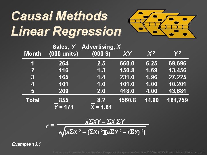
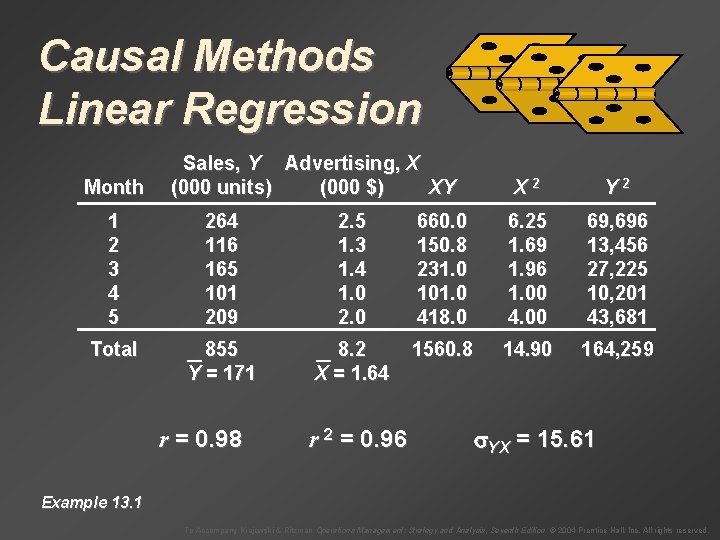
Causal Methods Linear Regression Month Sales, Y Advertising, X (000 units) (000 $) XY X 2 Y 2 1 2 3 4 5 264 116 165 101 209 2. 5 1. 3 1. 4 1. 0 2. 0 660. 0 150. 8 231. 0 101. 0 418. 0 6. 25 1. 69 1. 96 1. 00 4. 00 69, 696 13, 456 27, 225 10, 201 43, 681 Total 855 Y = 171 8. 2 X = 1. 64 1560. 8 14. 90 164, 259 r= n XY – X Y [n X 2 – ( X) 2][n Y 2 – ( Y) 2] Example 13. 1 To Accompany Krajewski & Ritzman Operations Management: Strategy and Analysis, Seventh Edition © 2004 Prentice Hall, Inc. All rights reserved.

Causal Methods Linear Regression Month Sales, Y Advertising, X (000 units) (000 $) XY X 2 Y 2 1 2 3 4 5 264 116 165 101 209 2. 5 1. 3 1. 4 1. 0 2. 0 660. 0 150. 8 231. 0 101. 0 418. 0 6. 25 1. 69 1. 96 1. 00 4. 00 69, 696 13, 456 27, 225 10, 201 43, 681 Total 855 Y = 171 8. 2 X = 1. 64 1560. 8 14. 90 164, 259 r = 0. 98 Example 13. 1 To Accompany Krajewski & Ritzman Operations Management: Strategy and Analysis, Seventh Edition © 2004 Prentice Hall, Inc. All rights reserved.

Causal Methods Linear Regression Month Sales, Y Advertising, X (000 units) (000 $) XY X 2 Y 2 1 2 3 4 5 264 116 165 101 209 2. 5 1. 3 1. 4 1. 0 2. 0 660. 0 150. 8 231. 0 101. 0 418. 0 6. 25 1. 69 1. 96 1. 00 4. 00 69, 696 13, 456 27, 225 10, 201 43, 681 Total 855 Y = 171 8. 2 X = 1. 64 1560. 8 14. 90 164, 259 r = 0. 98 r 2 = 0. 96 YX = 15. 61 Example 13. 1 To Accompany Krajewski & Ritzman Operations Management: Strategy and Analysis, Seventh Edition © 2004 Prentice Hall, Inc. All rights reserved.

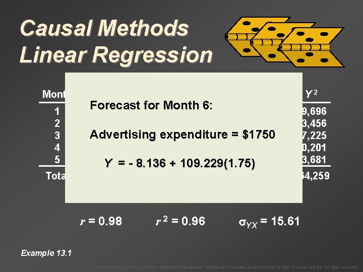
Causal Methods Linear Regression Month 1 2 3 4 5 Total Sales, Y Advertising, X (000 units) (000 $) XY Forecast for Month 6: 660. 0 264 2. 5 X 2 6. 25 116 1. 3 150. 8 1. 69 Advertising expenditure 165 1. 4 231. 0= $1750 1. 96 101 1. 0 101. 00 209 2. 0109. 229(1. 75) 418. 0 4. 00 Y = - 8. 136 + 855 Y = 171 r = 0. 98 8. 2 X = 1. 64 r 2 = 0. 96 1560. 8 14. 90 Y 2 69, 696 13, 456 27, 225 10, 201 43, 681 164, 259 YX = 15. 61 Example 13. 1 To Accompany Krajewski & Ritzman Operations Management: Strategy and Analysis, Seventh Edition © 2004 Prentice Hall, Inc. All rights reserved.

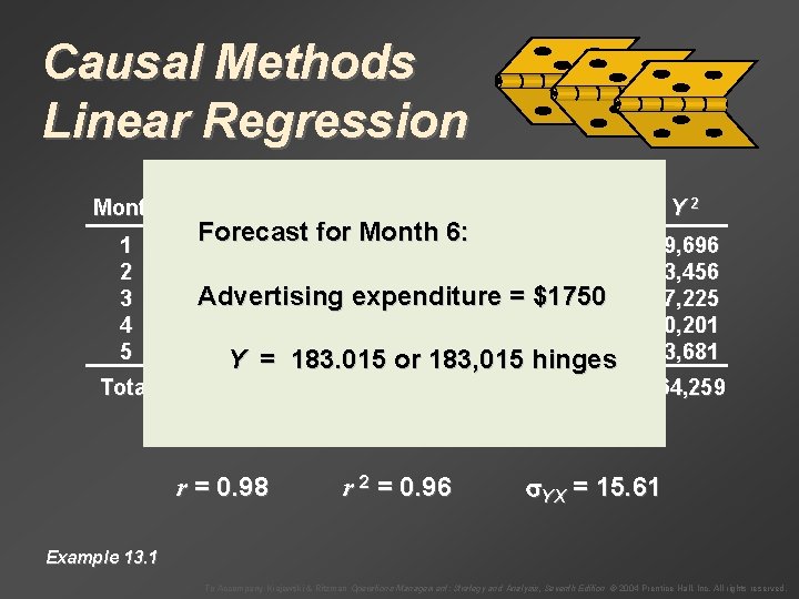
Causal Methods Linear Regression Month 1 2 3 4 5 Total Sales, Y Advertising, X (000 units) (000 $) XY Forecast for Month 6: 660. 0 264 2. 5 X 2 6. 25 116 1. 3 150. 8 1. 69 Advertising expenditure 165 1. 4 231. 0= $1750 1. 96 101 1. 0 101. 00 209 418. 0 hinges 4. 00 Y = 183. 0152. 0 or 183, 015 855 Y = 171 r = 0. 98 8. 2 X = 1. 64 r 2 = 0. 96 1560. 8 14. 90 Y 2 69, 696 13, 456 27, 225 10, 201 43, 681 164, 259 YX = 15. 61 Example 13. 1 To Accompany Krajewski & Ritzman Operations Management: Strategy and Analysis, Seventh Edition © 2004 Prentice Hall, Inc. All rights reserved.

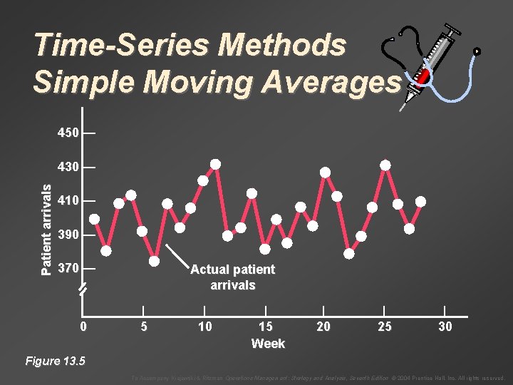
Time-Series Methods Simple Moving Averages 450 — Patient arrivals 430 — 410 — 390 — 370 — 0 Actual patient arrivals | 5 | 10 | 15 Week | 20 | 25 | 30 Figure 13. 5 To Accompany Krajewski & Ritzman Operations Management: Strategy and Analysis, Seventh Edition © 2004 Prentice Hall, Inc. All rights reserved.

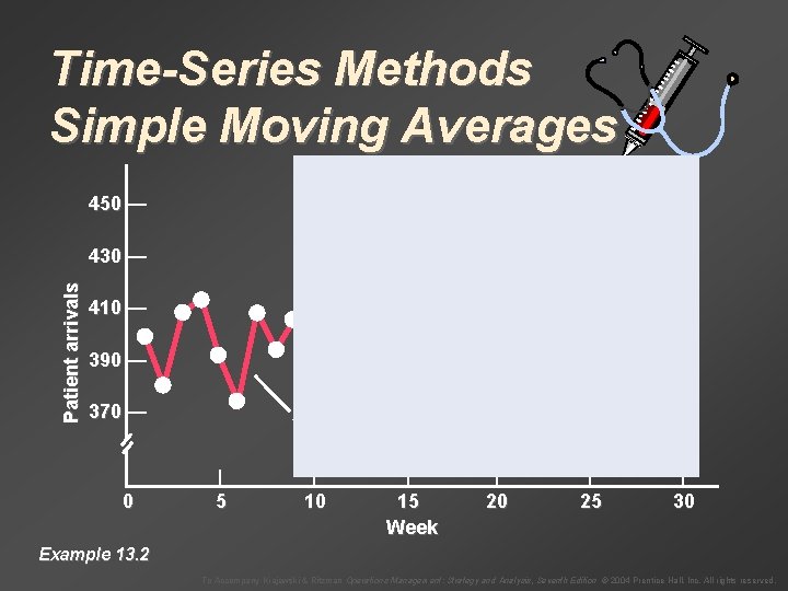
Time-Series Methods Simple Moving Averages 450 — Patient arrivals 430 — 410 — 390 — 370 — 0 Actual patient arrivals | 5 | 10 | 15 Week | 20 | 25 | 30 Example 13. 2 To Accompany Krajewski & Ritzman Operations Management: Strategy and Analysis, Seventh Edition © 2004 Prentice Hall, Inc. All rights reserved.

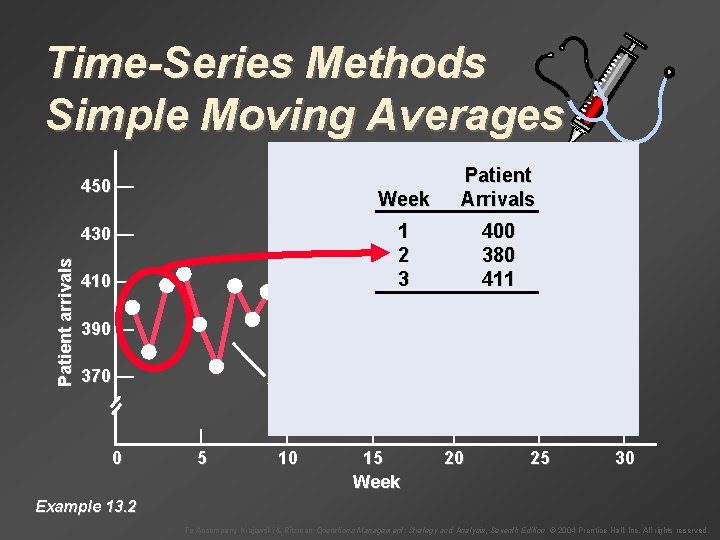
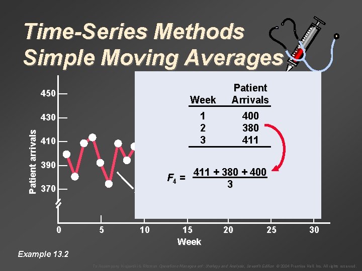
Time-Series Methods Simple Moving Averages 450 — Week Patient Arrivals 1 2 3 400 380 411 Patient arrivals 430 — 410 — 390 — 370 — 0 Actual patient arrivals | 5 | 10 | 15 Week | 20 | 25 | 30 Example 13. 2 To Accompany Krajewski & Ritzman Operations Management: Strategy and Analysis, Seventh Edition © 2004 Prentice Hall, Inc. All rights reserved.

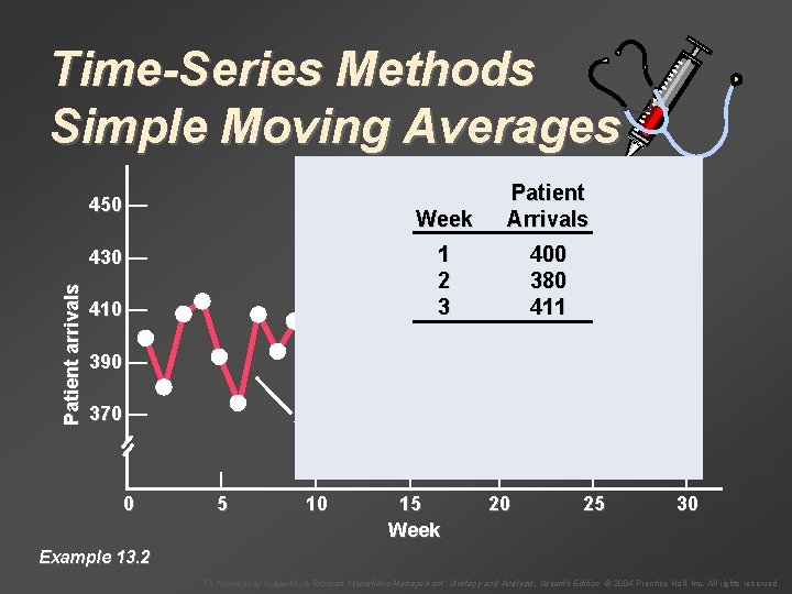
Time-Series Methods Simple Moving Averages 450 — Week Patient Arrivals 1 2 3 400 380 411 Patient arrivals 430 — 410 — 390 — 370 — 0 Actual patient arrivals | 5 | 10 | 15 Week | 20 | 25 | 30 Example 13. 2 To Accompany Krajewski & Ritzman Operations Management: Strategy and Analysis, Seventh Edition © 2004 Prentice Hall, Inc. All rights reserved.

Time-Series Methods Simple Moving Averages 450 — Week Patient Arrivals 1 2 3 400 380 411 Patient arrivals 430 — 410 — 390 — 411 + 380 + 400 F 4 = 3 Actual patient 370 — 0 Actual patient arrivals | 5 | 10 | 15 Week | 20 | 25 | 30 Example 13. 2 To Accompany Krajewski & Ritzman Operations Management: Strategy and Analysis, Seventh Edition © 2004 Prentice Hall, Inc. All rights reserved.

Time-Series Methods Simple Moving Averages 450 — Week Patient Arrivals 1 2 3 400 380 411 Patient arrivals 430 — 410 — 390 — F 4 = 397. 0 370 — 0 Actual patient arrivals | 5 | 10 | 15 Week | 20 | 25 | 30 Example 13. 2 To Accompany Krajewski & Ritzman Operations Management: Strategy and Analysis, Seventh Edition © 2004 Prentice Hall, Inc. All rights reserved.

Time-Series Methods Simple Moving Averages 450 — Week Patient Arrivals 1 2 3 400 380 411 Patient arrivals 430 — 410 — 390 — F 4 = 397. 0 370 — 0 Actual patient arrivals | 5 | 10 | 15 Week | 20 | 25 | 30 Example 13. 2 To Accompany Krajewski & Ritzman Operations Management: Strategy and Analysis, Seventh Edition © 2004 Prentice Hall, Inc. All rights reserved.

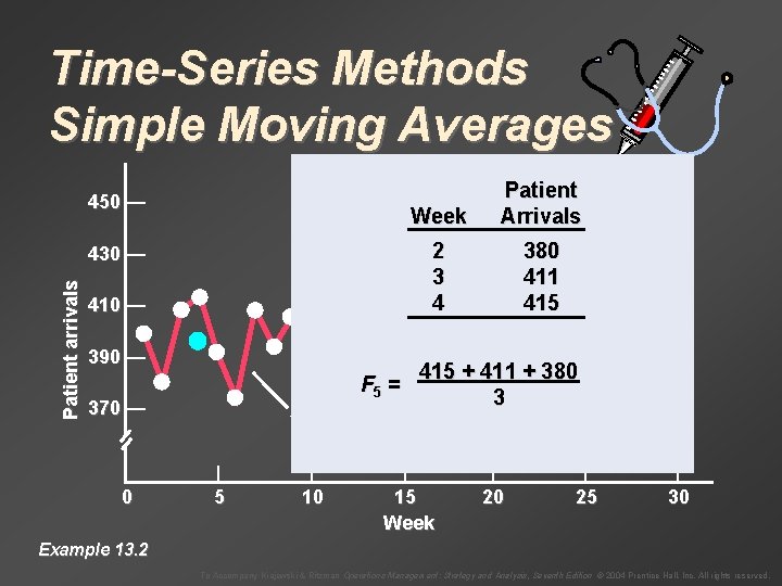
Time-Series Methods Simple Moving Averages 450 — Week Patient Arrivals 2 3 4 380 411 415 Patient arrivals 430 — 410 — 390 — F 5 = 370 — 0 415 + 411 + 380 3 Actual patient arrivals | 5 | 10 | 15 Week | 20 | 25 | 30 Example 13. 2 To Accompany Krajewski & Ritzman Operations Management: Strategy and Analysis, Seventh Edition © 2004 Prentice Hall, Inc. All rights reserved.

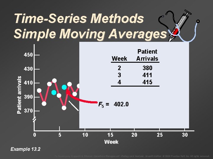
Time-Series Methods Simple Moving Averages 450 — Week Patient Arrivals 2 3 4 380 411 415 Patient arrivals 430 — 410 — 390 — F 5 = 402. 0 370 — 0 Actual patient arrivals | 5 | 10 | 15 Week | 20 | 25 | 30 Example 13. 2 To Accompany Krajewski & Ritzman Operations Management: Strategy and Analysis, Seventh Edition © 2004 Prentice Hall, Inc. All rights reserved.

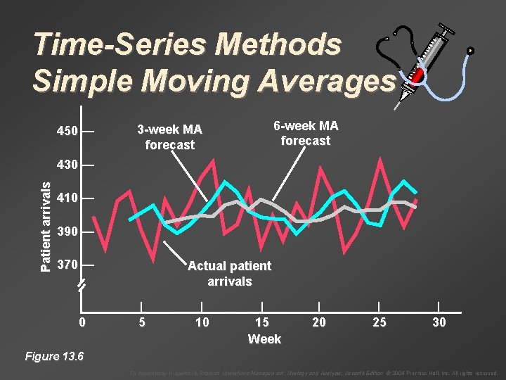
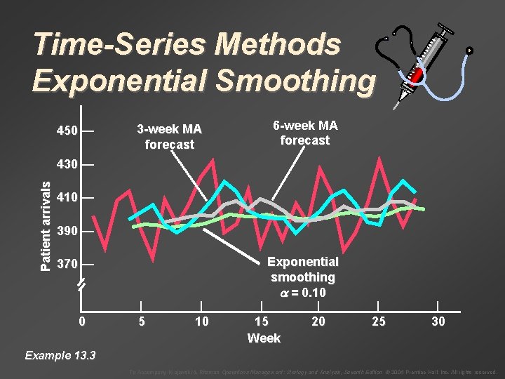
Time-Series Methods Simple Moving Averages 450 — 6 -week MA forecast 3 -week MA forecast Patient arrivals 430 — 410 — 390 — 370 — 0 Actual patient arrivals | 5 | 10 | 15 Week | 20 | 25 | 30 Figure 13. 6 To Accompany Krajewski & Ritzman Operations Management: Strategy and Analysis, Seventh Edition © 2004 Prentice Hall, Inc. All rights reserved.

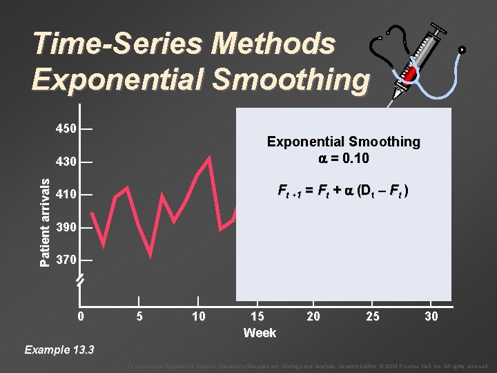
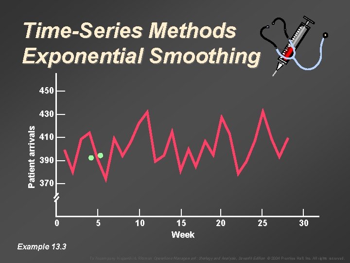
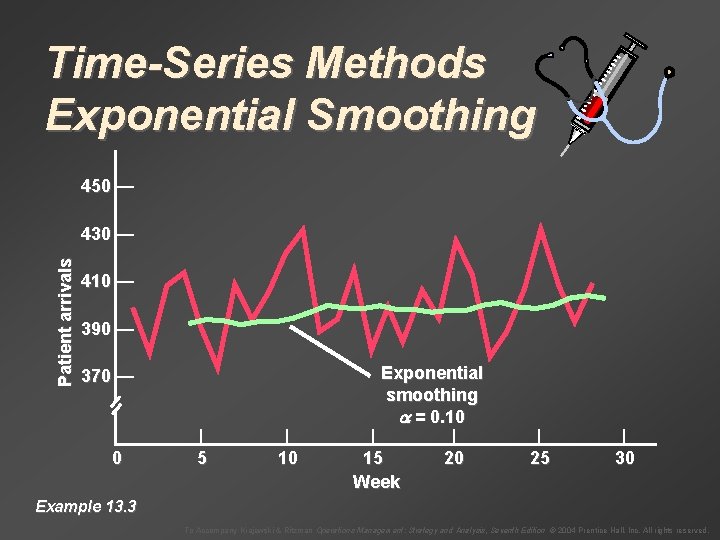
Time-Series Methods Exponential Smoothing Patient arrivals 450 — 430 — Exponential Smoothing = 0. 10 410 — Ft +1 = Ft + (Dt – Ft ) 390 — 370 — 0 | 5 | 10 | 15 Week | 20 | 25 | 30 Example 13. 3 To Accompany Krajewski & Ritzman Operations Management: Strategy and Analysis, Seventh Edition © 2004 Prentice Hall, Inc. All rights reserved.

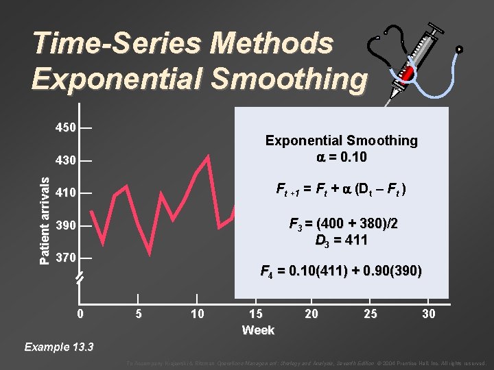
Time-Series Methods Exponential Smoothing Patient arrivals 450 — 430 — Exponential Smoothing = 0. 10 410 — Ft +1 = Ft + (Dt – Ft ) 390 — F 3 = (400 + 380)/2 D 3 = 411 370 — 0 F 4 = 0. 10(411) + 0. 90(390) | 5 | 10 | 15 Week | 20 | 25 | 30 Example 13. 3 To Accompany Krajewski & Ritzman Operations Management: Strategy and Analysis, Seventh Edition © 2004 Prentice Hall, Inc. All rights reserved.

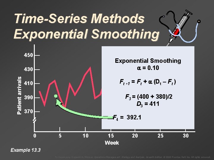
Time-Series Methods Exponential Smoothing Patient arrivals 450 — 430 — Exponential Smoothing = 0. 10 410 — Ft +1 = Ft + (Dt – Ft ) 390 — F 3 = (400 + 380)/2 D 3 = 411 370 — 0 F 4 = 392. 1 | 5 | 10 | 15 Week | 20 | 25 | 30 Example 13. 3 To Accompany Krajewski & Ritzman Operations Management: Strategy and Analysis, Seventh Edition © 2004 Prentice Hall, Inc. All rights reserved.

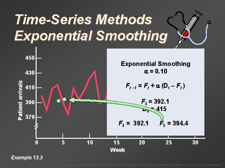
Time-Series Methods Exponential Smoothing Patient arrivals 450 — 430 — Exponential Smoothing = 0. 10 410 — Ft +1 = Ft + (Dt – Ft ) 390 — F 4 = 392. 1 D 4 = 415 370 — 0 F 4 = 392. 1 | 5 | 10 | 15 Week | 20 F 5 = 394. 4 | 25 | 30 Example 13. 3 To Accompany Krajewski & Ritzman Operations Management: Strategy and Analysis, Seventh Edition © 2004 Prentice Hall, Inc. All rights reserved.

Time-Series Methods Exponential Smoothing 450 — Patient arrivals 430 — 410 — 390 — 370 — 0 | 5 | 10 | 15 Week | 20 | 25 | 30 Example 13. 3 To Accompany Krajewski & Ritzman Operations Management: Strategy and Analysis, Seventh Edition © 2004 Prentice Hall, Inc. All rights reserved.

Time-Series Methods Exponential Smoothing 450 — Patient arrivals 430 — 410 — 390 — 370 — 0 | 5 | 10 Exponential smoothing = 0. 10 | | 15 20 Week | 25 | 30 Example 13. 3 To Accompany Krajewski & Ritzman Operations Management: Strategy and Analysis, Seventh Edition © 2004 Prentice Hall, Inc. All rights reserved.

Time-Series Methods Exponential Smoothing 450 — 3 -week MA forecast 6 -week MA forecast Patient arrivals 430 — 410 — 390 — 370 — 0 | 5 | 10 Exponential smoothing = 0. 10 | | 15 20 Week | 25 | 30 Example 13. 3 To Accompany Krajewski & Ritzman Operations Management: Strategy and Analysis, Seventh Edition © 2004 Prentice Hall, Inc. All rights reserved.

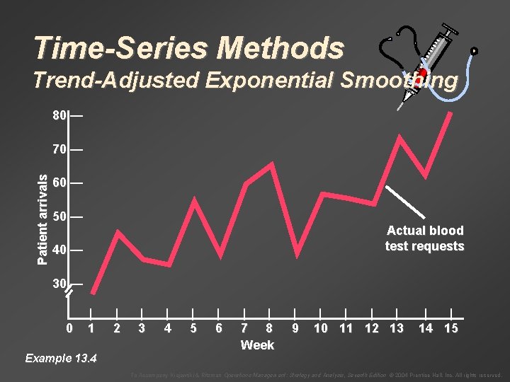
Time-Series Methods Trend-Adjusted Exponential Smoothing 80 — Patient arrivals 70 — 60 — 50 — Actual blood test requests 40 — 30 — 0 | 1 Example 13. 4 | 2 | 3 | 4 | 5 | 6 | | 7 8 Week | 9 | | 10 11 12 13 | | 14 15 To Accompany Krajewski & Ritzman Operations Management: Strategy and Analysis, Seventh Edition © 2004 Prentice Hall, Inc. All rights reserved.

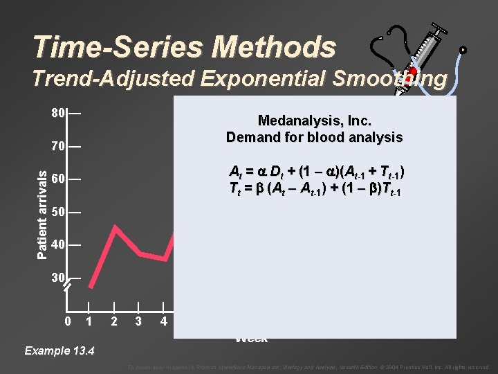
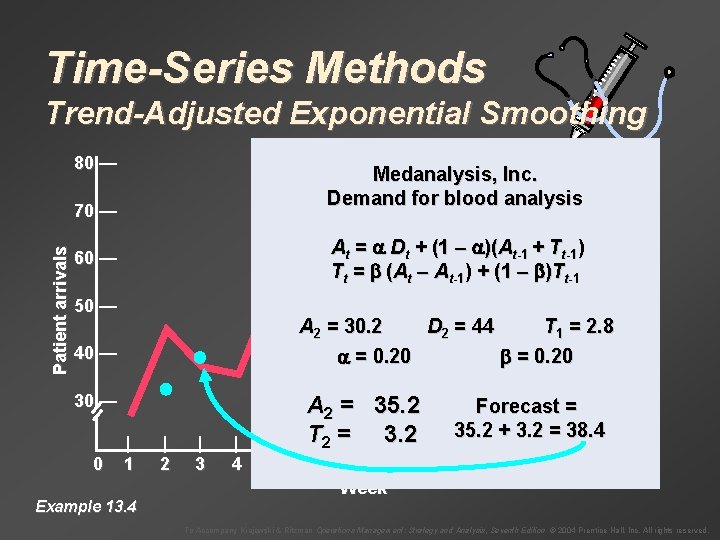
Time-Series Methods Trend-Adjusted Exponential Smoothing 80 — Medanalysis, Inc. Demand for blood analysis Patient arrivals 70 — At = Dt + (1 – )(At-1 + Tt-1) Tt = (At – At-1) + (1 – )Tt-1 60 — 50 — 40 — 30 — 0 | 1 Example 13. 4 | 2 | 3 | 4 | 5 | 6 | | 7 8 Week | 9 | | 10 11 12 13 | | 14 15 To Accompany Krajewski & Ritzman Operations Management: Strategy and Analysis, Seventh Edition © 2004 Prentice Hall, Inc. All rights reserved.

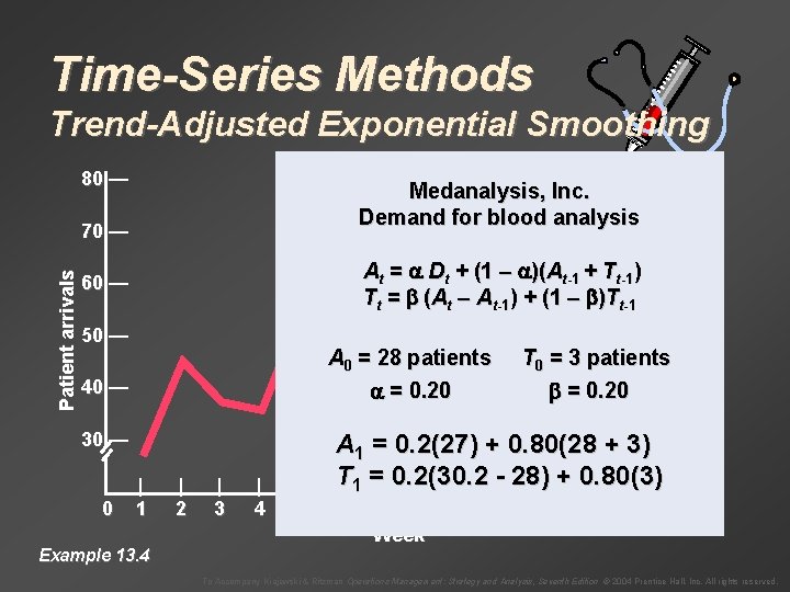
Time-Series Methods Trend-Adjusted Exponential Smoothing 80 — Medanalysis, Inc. Demand for blood analysis Patient arrivals 70 — At = Dt + (1 – )(At-1 + Tt-1) Tt = (At – At-1) + (1 – )Tt-1 60 — 50 — A 0 = 28 patients = 0. 20 40 — 30 — 0 | 1 Example 13. 4 | 2 | 3 | 4 | 5 T 0 = 3 patients = 0. 20 A 1 = 0. 2(27) + 0. 80(28 + 3) T | 1 =| 0. 2(30. 2 | | |- 28) | + |0. 80(3) | | 6 7 8 Week 9 10 11 12 13 | 14 15 To Accompany Krajewski & Ritzman Operations Management: Strategy and Analysis, Seventh Edition © 2004 Prentice Hall, Inc. All rights reserved.

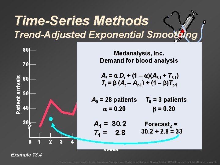
Time-Series Methods Trend-Adjusted Exponential Smoothing 80 — Medanalysis, Inc. Demand for blood analysis Patient arrivals 70 — At = Dt + (1 – )(At-1 + Tt-1) Tt = (At – At-1) + (1 – )Tt-1 60 — 50 — A 0 = 28 patients = 0. 20 40 — 30 — 0 | 1 Example 13. 4 | 2 | 3 | 4 | 5 A 1 = 30. 2 T 2. 8 | 1 =| | | 6 7 8 Week 9 T 0 = 3 patients = 0. 20 Forecast 2 = 30. 2 + 2. 8 = 33 | | 10 11 12 13 | | 14 15 To Accompany Krajewski & Ritzman Operations Management: Strategy and Analysis, Seventh Edition © 2004 Prentice Hall, Inc. All rights reserved.

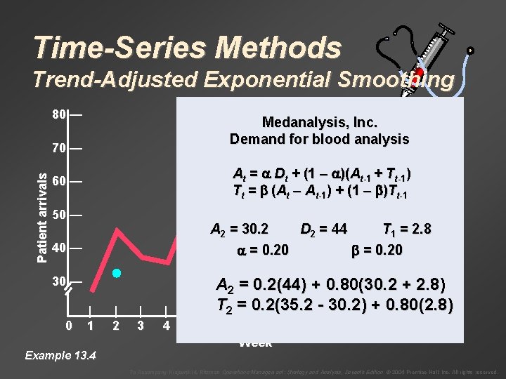
Time-Series Methods Trend-Adjusted Exponential Smoothing 80 — Medanalysis, Inc. Demand for blood analysis Patient arrivals 70 — At = Dt + (1 – )(At-1 + Tt-1) Tt = (At – At-1) + (1 – )Tt-1 60 — 50 — A 2 = 30. 2 D 2 = 44 T 1 = 2. 8 = 0. 20 40 — 30 — 0 | 1 Example 13. 4 | 2 | 3 | 4 | 5 A 2 = 0. 2(44) + 0. 80(30. 2 + 2. 8) |T 2 =| 0. 2(35. 2 | | |- 30. 2) | |+ 0. 80(2. 8) | | | 6 7 8 Week 9 10 11 12 13 14 15 To Accompany Krajewski & Ritzman Operations Management: Strategy and Analysis, Seventh Edition © 2004 Prentice Hall, Inc. All rights reserved.

Time-Series Methods Trend-Adjusted Exponential Smoothing 80 — Medanalysis, Inc. Demand for blood analysis Patient arrivals 70 — At = Dt + (1 – )(At-1 + Tt-1) Tt = (At – At-1) + (1 – )Tt-1 60 — 50 — A 2 = 30. 2 D 2 = 44 T 1 = 2. 8 = 0. 20 40 — 30 — 0 | 1 Example 13. 4 | 2 | 3 | 4 | 5 A 2 = 35. 2 |T 2 =| | 3. 2| 6 7 8 Week 9 Forecast = 35. 2 + 3. 2 = 38. 4 | | 10 11 12 13 | | 14 15 To Accompany Krajewski & Ritzman Operations Management: Strategy and Analysis, Seventh Edition © 2004 Prentice Hall, Inc. All rights reserved.

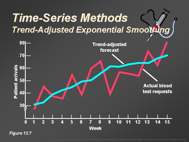
Time-Series Methods Trend-Adjusted Exponential Smoothing 80 — Trend-adjusted forecast Patient arrivals 70 — 60 — 50 — Actual blood test requests 40 — 30 — 0 Figure 13. 7 | 1 | 2 | 3 | 4 | 5 | 6 | | 7 8 Week | 9 | | 10 11 12 13 | | 14 15 To Accompany Krajewski & Ritzman Operations Management: Strategy and Analysis, Seventh Edition © 2004 Prentice Hall, Inc. All rights reserved.

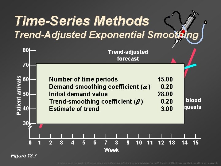
Time-Series Methods Trend-Adjusted Exponential Smoothing 80 — Trend-adjusted forecast Patient arrivals 70 — Number of time periods Demand smoothing coefficient ( ) Initial demand value Trend-smoothing coefficient ( ) Estimate of trend 60 — 50 — 40 — 15. 00 0. 20 28. 00 Actual blood 0. 20 test requests 3. 00 30 — 0 Figure 13. 7 | 1 | 2 | 3 | 4 | 5 | 6 | | 7 8 Week | 9 | | 10 11 12 13 | | 14 15 To Accompany Krajewski & Ritzman Operations Management: Strategy and Analysis, Seventh Edition © 2004 Prentice Hall, Inc. All rights reserved.

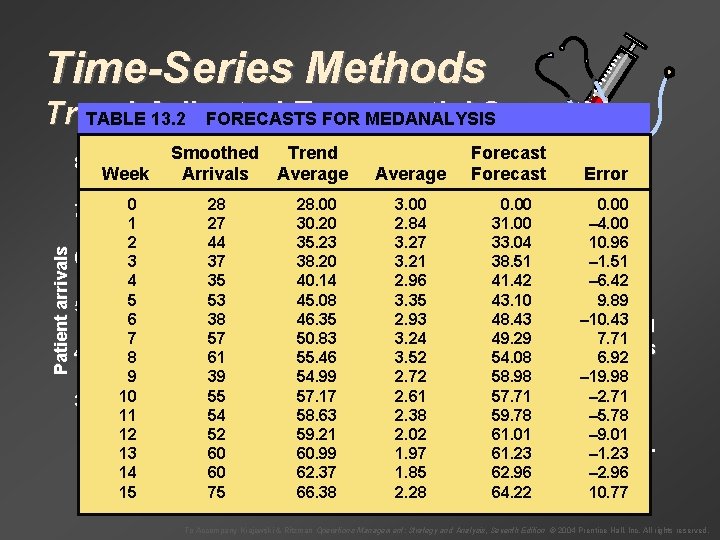
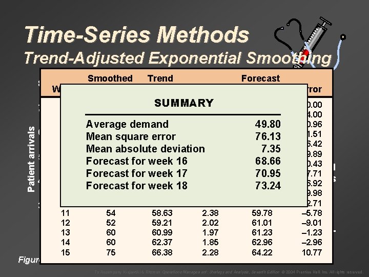
Time-Series Methods Trend-Adjusted Exponential Smoothing TABLE 13. 2 FORECASTS FOR MEDANALYSIS Smoothed Arrivals 80 — Week Patient arrivals 70 — 0 1 2 60 — 3 4 50 — 5 6 7 40 — 8 9 30 — 10 11 12 | 13 0 14 1 15 | 2 28 27 44 37 35 53 38 57 61 39 55 54 | 52 | 60 3 60 4 75 Trend Forecast Average Trend-adjusted Average Forecast forecast | 5 28. 00 30. 20 35. 23 38. 20 40. 14 45. 08 46. 35 50. 83 55. 46 54. 99 57. 17 58. 63 59. 21 | | | 60. 99 6 7 8 62. 37 66. 38 Week 3. 00 2. 84 3. 27 3. 21 2. 96 3. 35 2. 93 3. 24 3. 52 2. 72 2. 61 2. 38 2. 02 | 1. 97 9 1. 85 2. 28 Error 0. 00 31. 00 – 4. 00 33. 04 10. 96 38. 51 – 1. 51 41. 42 – 6. 42 43. 10 9. 89 48. 43 Actual – 10. 43 blood 49. 29 7. 71 test requests 54. 08 6. 92 58. 98 – 19. 98 57. 71 – 2. 71 59. 78 – 5. 78 | | 61. 01 | | – 9. 01 | | 61. 23 – 1. 23 10 1162. 96 12 13 – 2. 96 14 15 64. 22 10. 77 To Accompany Krajewski & Ritzman Operations Management: Strategy and Analysis, Seventh Edition © 2004 Prentice Hall, Inc. All rights reserved.

Time-Series Methods Trend-Adjusted Exponential Smoothing 80 — Week 70 — 0 Patient arrivals 1 2 60 — 3 4 50 — 5 6 7 40 — 8 9 30 — 10 11 12 | 13 0 14 1 15 Figure 13. 7 Smoothed Arrivals Trend Forecast Average Trend-adjusted Average Forecast forecast SUMMARY 28 28. 00 3. 00 27 30. 20 2. 84 44 35. 23 3. 27 Average demand 37 square error 38. 20 3. 21 Mean 35 40. 14 2. 96 Mean absolute deviation 53 45. 08 3. 35 Forecast for week 38 46. 35 16 2. 93 57 50. 83 17 3. 24 Forecast for week 61 55. 46 18 3. 52 Forecast for week 39 54. 99 2. 72 55 57. 17 2. 61 54 58. 63 2. 38 | | 52 | | 59. 21 | | | 2. 02 | 60 60. 99 1. 97 2 3 60 4 5 62. 37 6 7 8 1. 85 9 75 66. 38 Week 2. 28 Error 0. 00 31. 00 – 4. 00 33. 04 10. 96 49. 80 38. 51 – 1. 51 76. 13 41. 42 – 6. 42 7. 35 43. 10 9. 89 68. 66 48. 43 – 10. 43 Actual blood 49. 29 7. 71 70. 95 test requests 54. 08 6. 92 73. 24 58. 98 – 19. 98 57. 71 – 2. 71 59. 78 – 5. 78 | | 61. 01 | | – 9. 01 | | 61. 23 – 1. 23 10 1162. 96 12 13 – 2. 96 14 15 64. 22 10. 77 To Accompany Krajewski & Ritzman Operations Management: Strategy and Analysis, Seventh Edition © 2004 Prentice Hall, Inc. All rights reserved.

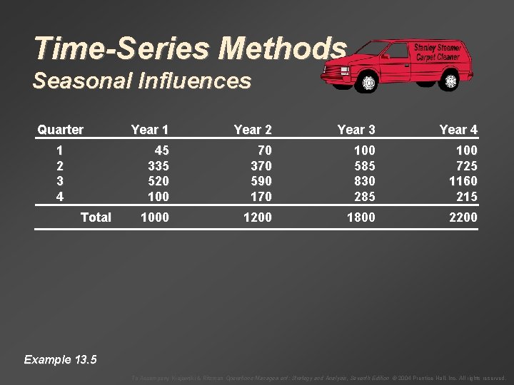
Time-Series Methods Seasonal Influences Quarter 1 2 3 4 Total Year 1 Year 2 Year 3 Year 4 45 335 520 100 70 370 590 170 100 585 830 285 100 725 1160 215 1000 1200 1800 2200 Example 13. 5 To Accompany Krajewski & Ritzman Operations Management: Strategy and Analysis, Seventh Edition © 2004 Prentice Hall, Inc. All rights reserved.

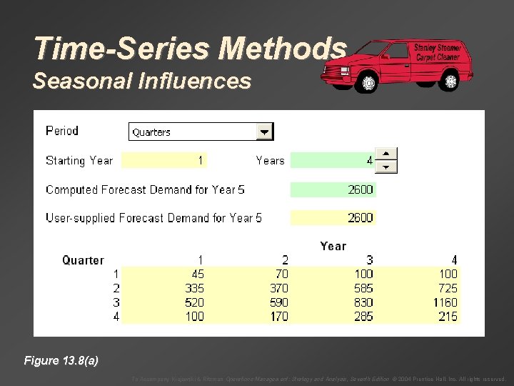
Time-Series Methods Seasonal Influences Figure 13. 8(a) To Accompany Krajewski & Ritzman Operations Management: Strategy and Analysis, Seventh Edition © 2004 Prentice Hall, Inc. All rights reserved.

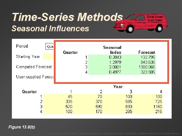
Time-Series Methods Seasonal Influences Figure 13. 8(b) To Accompany Krajewski & Ritzman Operations Management: Strategy and Analysis, Seventh Edition © 2004 Prentice Hall, Inc. All rights reserved.

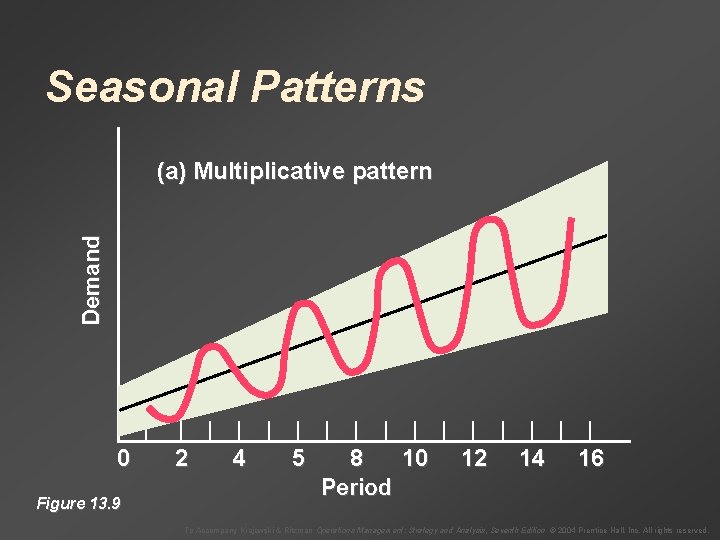
Seasonal Patterns Demand (a) Multiplicative pattern | 0 Figure 13. 9 | | | | 2 4 5 8 10 12 14 16 Period To Accompany Krajewski & Ritzman Operations Management: Strategy and Analysis, Seventh Edition © 2004 Prentice Hall, Inc. All rights reserved.

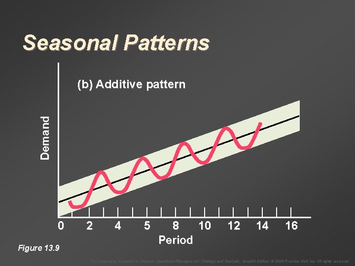
Seasonal Patterns Demand (b) Additive pattern | 0 Figure 13. 9 | | | | 2 4 5 8 10 12 14 16 Period To Accompany Krajewski & Ritzman Operations Management: Strategy and Analysis, Seventh Edition © 2004 Prentice Hall, Inc. All rights reserved.

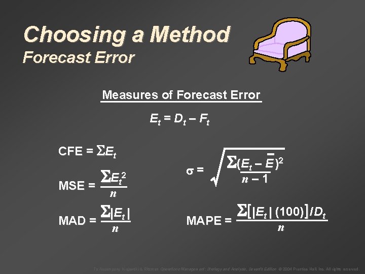
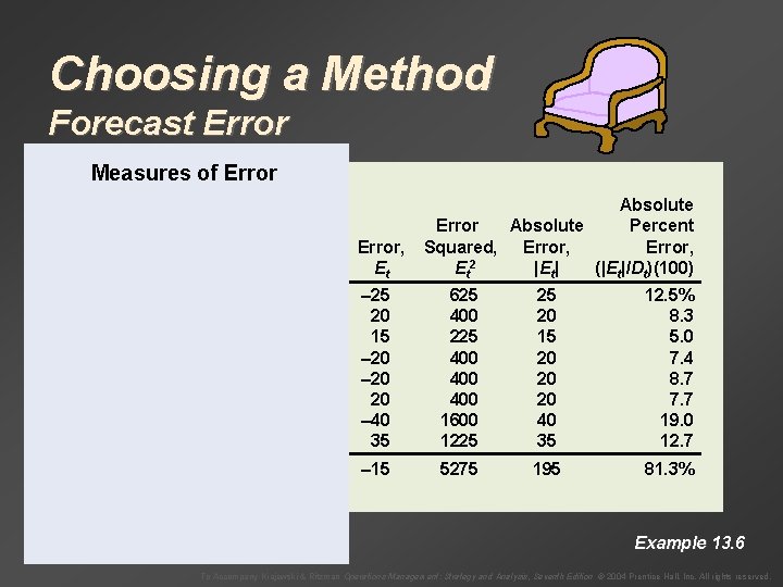
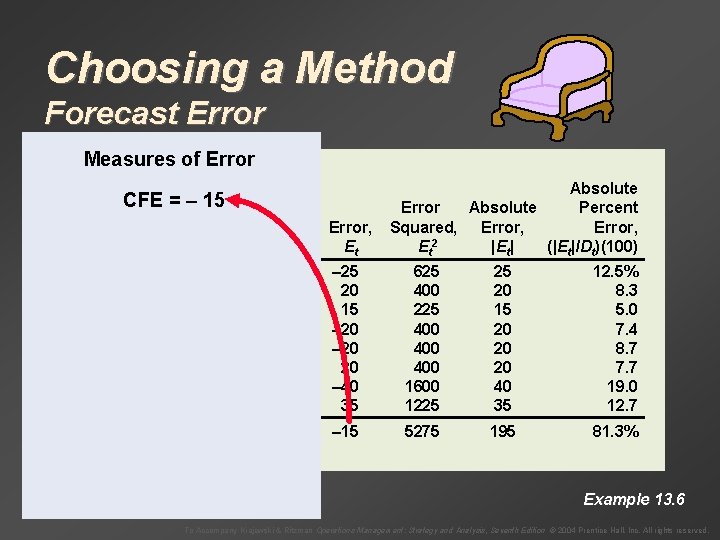
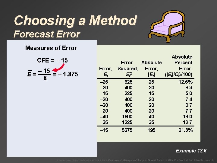
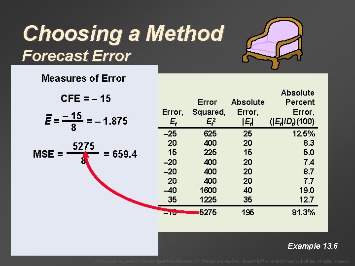
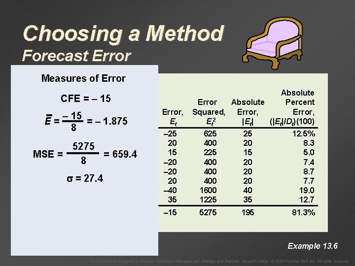
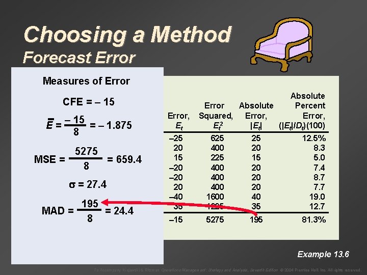
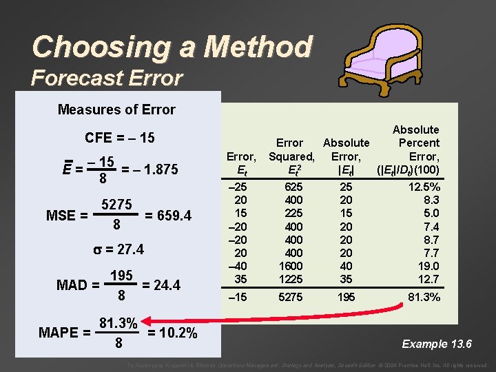
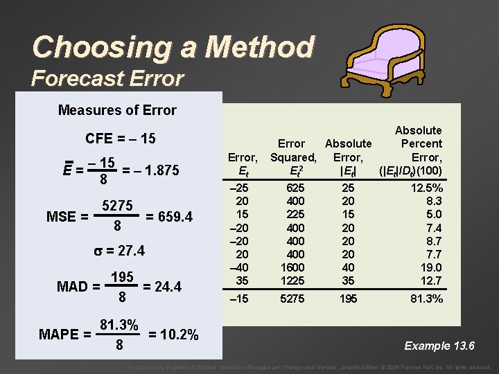
Choosing a Method Forecast Error Measures of Forecast Error E t = Dt – F t CFE = Et MSE = E t 2 = (E t – E )2 n |Et | MAD = n MAPE = n– 1 [ |Et | (100) ] / Dt n To Accompany Krajewski & Ritzman Operations Management: Strategy and Analysis, Seventh Edition © 2004 Prentice Hall, Inc. All rights reserved.

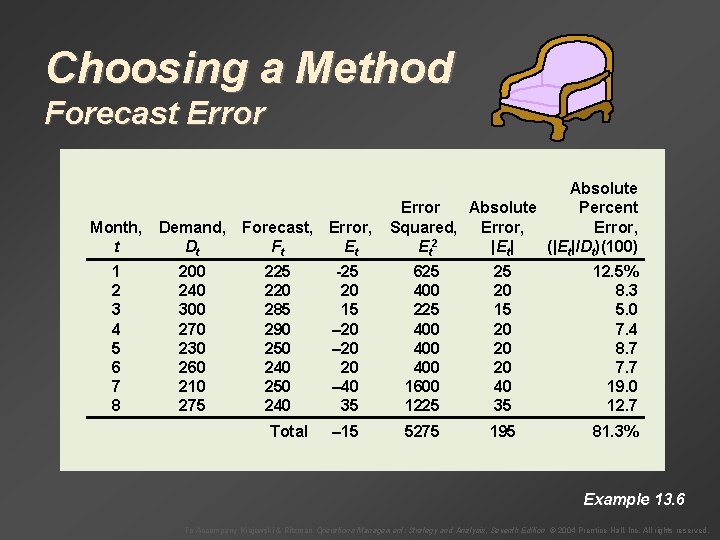
Choosing a Method Forecast Error Month, Demand, t Dt 1 2 3 4 5 6 7 8 200 240 300 270 230 260 210 275 Forecast, Error, Ft Et 225 220 285 290 250 240 Total Absolute Error Absolute Percent Squared, Error, 2 Et |Et| (|Et|/Dt)(100) -25 20 15 – 20 20 – 40 35 625 400 225 400 400 1600 1225 25 20 15 20 20 20 40 35 12. 5% 8. 3 5. 0 7. 4 8. 7 7. 7 19. 0 12. 7 – 15 5275 195 81. 3% Example 13. 6 To Accompany Krajewski & Ritzman Operations Management: Strategy and Analysis, Seventh Edition © 2004 Prentice Hall, Inc. All rights reserved.

Choosing a Method Forecast Error Measures of Error Month, Demand, t Dt 1 2 3 4 5 6 7 8 200 240 300 270 230 260 210 275 Forecast, Error, Ft Et 225 220 285 290 250 240 Total Absolute Error Absolute Percent Squared, Error, 2 Et |Et| (|Et|/Dt)(100) – 25 20 15 – 20 20 – 40 35 625 400 225 400 400 1600 1225 25 20 15 20 20 20 40 35 12. 5% 8. 3 5. 0 7. 4 8. 7 7. 7 19. 0 12. 7 – 15 5275 195 81. 3% Example 13. 6 To Accompany Krajewski & Ritzman Operations Management: Strategy and Analysis, Seventh Edition © 2004 Prentice Hall, Inc. All rights reserved.

Choosing a Method Forecast Error Measures of Error CFE = – 15 Month, Demand, t Dt 1 2 3 4 5 6 7 8 200 240 300 270 230 260 210 275 Forecast, Error, Ft Et 225 220 285 290 250 240 Total Absolute Error Absolute Percent Squared, Error, 2 Et |Et| (|Et|/Dt)(100) – 25 20 15 – 20 20 – 40 35 625 400 225 400 400 1600 1225 25 20 15 20 20 20 40 35 12. 5% 8. 3 5. 0 7. 4 8. 7 7. 7 19. 0 12. 7 – 15 5275 195 81. 3% Example 13. 6 To Accompany Krajewski & Ritzman Operations Management: Strategy and Analysis, Seventh Edition © 2004 Prentice Hall, Inc. All rights reserved.

Choosing a Method Forecast Error Measures of Error CFE = – 15 Month, Demand, Forecast, Error, – 15 Et E =t =D–t 1. 875 Ft 1 2 3 4 5 6 7 8 8 200 240 300 270 230 260 210 275 220 285 290 250 240 Total Absolute Error Absolute Percent Squared, Error, 2 Et |Et| (|Et|/Dt)(100) – 25 20 15 – 20 20 – 40 35 625 400 225 400 400 1600 1225 25 20 15 20 20 20 40 35 12. 5% 8. 3 5. 0 7. 4 8. 7 7. 7 19. 0 12. 7 – 15 5275 195 81. 3% Example 13. 6 To Accompany Krajewski & Ritzman Operations Management: Strategy and Analysis, Seventh Edition © 2004 Prentice Hall, Inc. All rights reserved.

Choosing a Method Forecast Error Measures of Error CFE = – 15 Month, Demand, Forecast, Error, – 15 Et E =t =D–t 1. 875 Ft 1 2 MSE 3= 4 5 6 7 8 8 200 240 5275 300 = 8 270 230 260 210 275 220 285 659. 4 290 250 240 Total Absolute Error Absolute Percent Squared, Error, 2 Et |Et| (|Et|/Dt)(100) – 25 20 15 – 20 20 – 40 35 625 400 225 400 400 1600 1225 25 20 15 20 20 20 40 35 12. 5% 8. 3 5. 0 7. 4 8. 7 7. 7 19. 0 12. 7 – 15 5275 195 81. 3% Example 13. 6 To Accompany Krajewski & Ritzman Operations Management: Strategy and Analysis, Seventh Edition © 2004 Prentice Hall, Inc. All rights reserved.

Choosing a Method Forecast Error Measures of Error CFE = – 15 Month, Demand, Forecast, Error, – 15 Et E =t =D–t 1. 875 Ft 1 2 MSE 3= 4 5 6 7 8 8 200 240 5275 300 = 8 270 230 = 27. 4 260 210 275 220 285 659. 4 290 250 240 Total Absolute Error Absolute Percent Squared, Error, 2 Et |Et| (|Et|/Dt)(100) – 25 20 15 – 20 20 – 40 35 625 400 225 400 400 1600 1225 25 20 15 20 20 20 40 35 12. 5% 8. 3 5. 0 7. 4 8. 7 7. 7 19. 0 12. 7 – 15 5275 195 81. 3% Example 13. 6 To Accompany Krajewski & Ritzman Operations Management: Strategy and Analysis, Seventh Edition © 2004 Prentice Hall, Inc. All rights reserved.

Choosing a Method Forecast Error Measures of Error CFE = – 15 Month, Demand, Forecast, Error, – 15 Et E =t =D–t 1. 875 Ft 1 2 MSE 3= 4 5 6 7 8 8 200 240 5275 300 = 8 270 230 = 27. 4 260 210 195 275 MAD = 8 225 220 285 659. 4 290 250 240 = 24. 4 Total Absolute Error Absolute Percent Squared, Error, 2 Et |Et| (|Et|/Dt)(100) – 25 20 15 – 20 20 – 40 35 625 400 225 400 400 1600 1225 25 20 15 20 20 20 40 35 12. 5% 8. 3 5. 0 7. 4 8. 7 7. 7 19. 0 12. 7 – 15 5275 195 81. 3% Example 13. 6 To Accompany Krajewski & Ritzman Operations Management: Strategy and Analysis, Seventh Edition © 2004 Prentice Hall, Inc. All rights reserved.

Choosing a Method Forecast Error Measures of Error CFE = – 15 Month, Demand, Forecast, Error, – 15 Et E =t =D–t 1. 875 Ft 1 2 MSE 3= 4 5 6 7 8 8 200 240 5275 300 = 8 270 230 = 27. 4 260 210 195 275 MAD = 8 225 220 285 659. 4 290 250 240 = 24. 4 Total 81. 3% MAPE = = 10. 2% 8 Absolute Error Absolute Percent Squared, Error, 2 Et |Et| (|Et|/Dt)(100) – 25 20 15 – 20 20 – 40 35 625 400 225 400 400 1600 1225 25 20 15 20 20 20 40 35 12. 5% 8. 3 5. 0 7. 4 8. 7 7. 7 19. 0 12. 7 – 15 5275 195 81. 3% Example 13. 6 To Accompany Krajewski & Ritzman Operations Management: Strategy and Analysis, Seventh Edition © 2004 Prentice Hall, Inc. All rights reserved.

Choosing a Method Forecast Error Measures of Error CFE = – 15 Month, Demand, Forecast, Error, – 15 Et E =t =D–t 1. 875 Ft 1 2 MSE 3= 4 5 6 7 8 8 200 240 5275 300 = 8 270 230 = 27. 4 260 210 195 275 MAD = 8 225 220 285 659. 4 290 250 240 = 24. 4 Total 81. 3% MAPE = = 10. 2% 8 Absolute Error Absolute Percent Squared, Error, 2 Et |Et| (|Et|/Dt)(100) – 25 20 15 – 20 20 – 40 35 625 400 225 400 400 1600 1225 25 20 15 20 20 20 40 35 12. 5% 8. 3 5. 0 7. 4 8. 7 7. 7 19. 0 12. 7 – 15 5275 195 81. 3% Example 13. 6 To Accompany Krajewski & Ritzman Operations Management: Strategy and Analysis, Seventh Edition © 2004 Prentice Hall, Inc. All rights reserved.

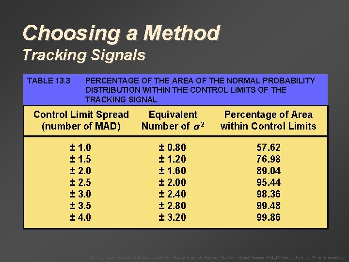
Choosing a Method Tracking Signals TABLE 13. 3 PERCENTAGE OF THE AREA OF THE NORMAL PROBABILITY DISTRIBUTION WITHIN THE CONTROL LIMITS OF THE TRACKING SIGNAL Control Limit Spread (number of MAD) Equivalent Number of 2 Percentage of Area within Control Limits ± 1. 0 ± 1. 5 ± 2. 0 ± 2. 5 ± 3. 0 ± 3. 5 ± 4. 0 ± 0. 80 ± 1. 20 ± 1. 60 ± 2. 00 ± 2. 40 ± 2. 80 ± 3. 20 57. 62 76. 98 89. 04 95. 44 98. 36 99. 48 99. 86 To Accompany Krajewski & Ritzman Operations Management: Strategy and Analysis, Seventh Edition © 2004 Prentice Hall, Inc. All rights reserved.

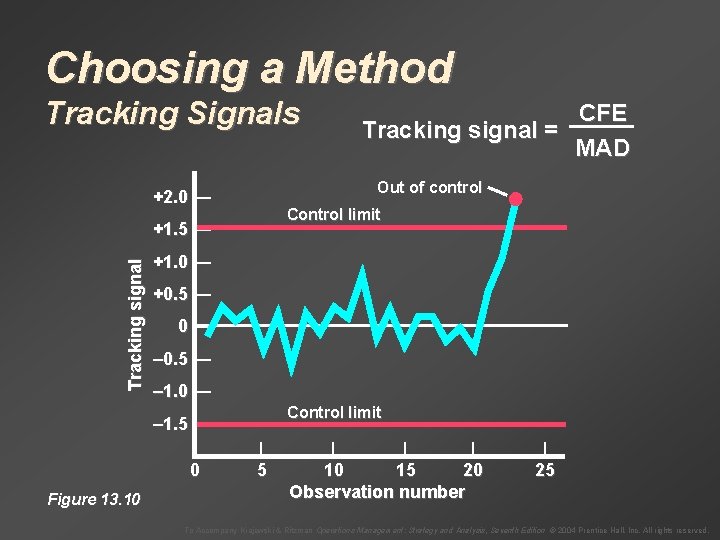
Choosing a Method Tracking Signals Out of control +2. 0 — Control limit Tracking signal +1. 5 — +1. 0 — +0. 5 — 0— – 0. 5 — – 1. 0 — Control limit – 1. 5 — 0 Figure 13. 10 CFE Tracking signal = MAD | 5 | | | 10 15 20 Observation number | 25 To Accompany Krajewski & Ritzman Operations Management: Strategy and Analysis, Seventh Edition © 2004 Prentice Hall, Inc. All rights reserved.

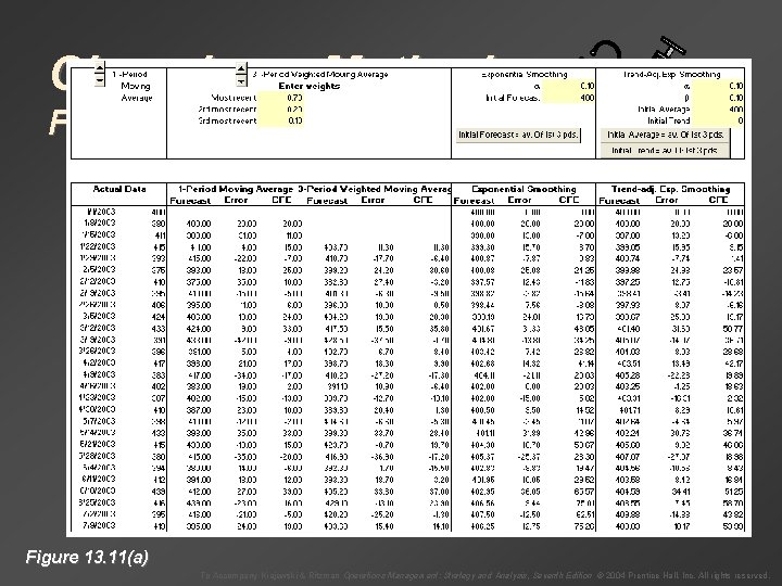
Choosing a Method Forecast Error Figure 13. 11(a) To Accompany Krajewski & Ritzman Operations Management: Strategy and Analysis, Seventh Edition © 2004 Prentice Hall, Inc. All rights reserved.

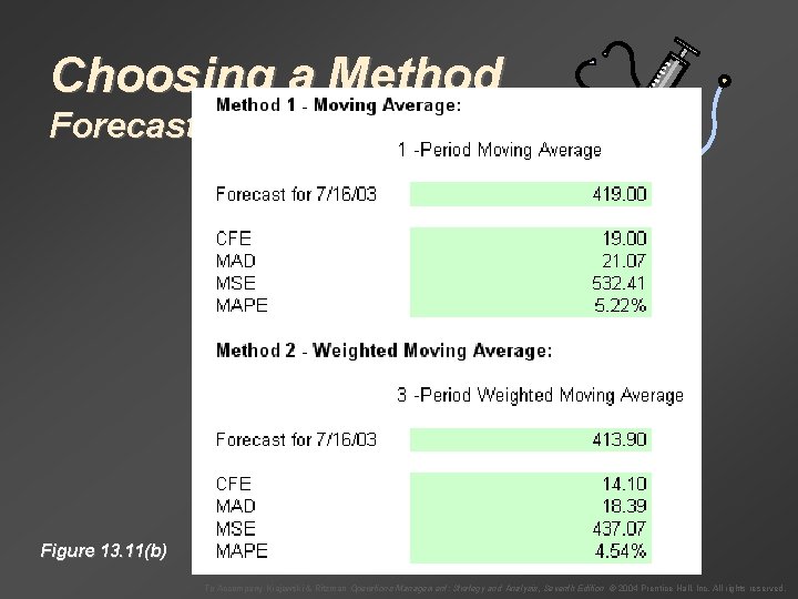
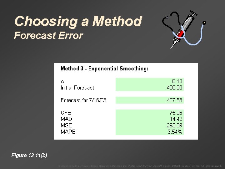
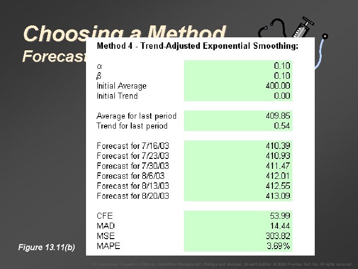
Choosing a Method Forecast Error Figure 13. 11(b) To Accompany Krajewski & Ritzman Operations Management: Strategy and Analysis, Seventh Edition © 2004 Prentice Hall, Inc. All rights reserved.

Choosing a Method Forecast Error Figure 13. 11(b) To Accompany Krajewski & Ritzman Operations Management: Strategy and Analysis, Seventh Edition © 2004 Prentice Hall, Inc. All rights reserved.

Choosing a Method Forecast Error Figure 13. 11(b) To Accompany Krajewski & Ritzman Operations Management: Strategy and Analysis, Seventh Edition © 2004 Prentice Hall, Inc. All rights reserved.

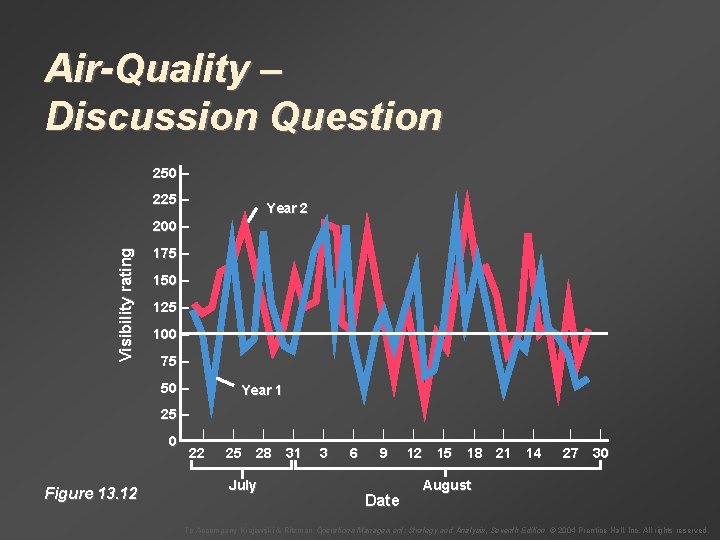
Air-Quality – Discussion Question 250 – 225 – Year 2 Visibility rating 200 – 175 – 150 – 125 – 100 – 75 – 50 – Year 1 25 – 0 Figure 13. 12 | 22 | | | 25 28 31 July | 3 | 6 | 9 Date | | | 12 15 18 21 14 | | 27 30 August To Accompany Krajewski & Ritzman Operations Management: Strategy and Analysis, Seventh Edition © 2004 Prentice Hall, Inc. All rights reserved.