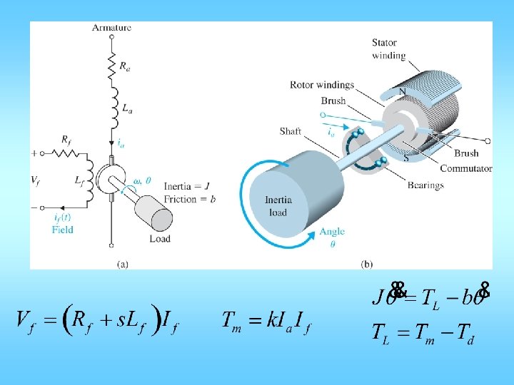
For field control with constant armature current For

For field control with constant armature current For armature control with constant field current

Armature controlled motor in feedback

Get TF from wd to w and Td to w.

DC Motor Driving an Inertial Load

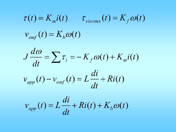
• • w(t): angular rate of the load, output vapp(t): applied voltage, the input i(t) armature current vemf(t) back emf voltage generated by the motor rotation – vemf(t) = constant * motor velocity • t(t): mechanical torque generated by the motor – t(t) = constant * armature current

State Space model

Matlab R= 2. 0; % Ohms L= 0. 5; % Henrys Km =. 015; % torque constant Kb =. 015; % emf constant Kf = 0. 2; % Nms J= 0. 02 % kg. m^2; A = [-R/L -Kb/L; Km/J -Kf/J]; B = [1/L; 0]; C = [0 1]; D = [0]; sys_dc = ss(A, B, C, D)

Matlab output a= b= c= d= x 1 x 2 x 1 -4 0. 75 x 1 x 2 u 1 2 0 y 1 x 1 0 y 1 u 1 0 x 2 -0. 03 -10 x 2 1

SS to TF or ZPK representation >> sys_tf = tf(sys_dc) Transfer function: 1. 5 ------------s^2 + 14 s + 40. 02 >> sys_zpk = zpk(sys_dc) Zero/pole/gain: 1. 5 ------------(s+4. 004) (s+9. 996)

• Note: The state-space representation is best suited for numerical computations. For highest accuracy, convert to state space prior to combining models and avoid the transfer function and zero/pole/gain representations, except for model specification and inspection.

4 ways to enter system model sys sys = = tf(num, den) % Transfer function zpk(z, p, k) % Zero/pole/gain ss(a, b, c, d) % State-space frd(response, frequencies) % Frequency response data s = tf('s'); sys_tf = 1. 5/(s^2+14*s+40. 02) Transfer function: 1. 5 ------------s^2 + 14 s + 40. 02 sys_tf = tf(1. 5, [1 14 40. 02])

4 ways to enter system model sys_zpk = zpk([], [-9. 996 -4. 004], 1. 5) Zero/pole/gain: 1. 5 ------------(s+9. 996) (s+4. 004)

Modeling • Types of systems electric mechanical electromechanical fluid systems thermal systems • Types of models I/O o. d. e. models Transfer Function state space models

I/O o. d. e. model: o. d. e. involving input/output only. linear: where u: input y: output

State space model: linear: or in some text: where: u: input y: output x: state vector A, B, C, D, or F, G, H, J are const matrices

Other types of models: Transfer function model (This is I/O model) from I/O o. d. e. model, take Laplace transform:

Then I/O ODE model in L. T. domain becomes: denote or

ODE or TF to SS

State space model to T. F. / block diagram: s. s. Take L. T. : From 1 s. X(s)-AX(s)=BU(s) s. IX(s)-AX(s)=BU(s) (s. I-A)X(s)=BU(s) X(s)=(s. I-A)-1 BU(s) 1 2

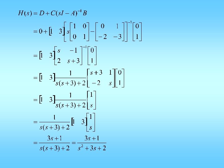
into 2 : Y(s)=C(s. I-A)-1 BU(s)+DU(s) Y(s)=[C(s. I-A)-1 B+D] U(s) H(s)= D+C(s. I-A)-1 B is the T. F. from u to y from 1

Example

>> n=[1 2 3]; d=[1 4 5 6]; >> [A, B, C, D]=tf 2 ss(n, d) • In Matlab: >> A=[0 1; -2 -3]; >> B=[0; 1]; >> C=[1 3]; >> D=[0]; >> [n, d]=ss 2 tf(A, B, C, D) n= 0 d= 1 3. 0000 3 2 1. 0000 A= -4 1 0 -5 0 1 -6 0 0 2 3 B= 1 0 0 C= 1 D= 0 >> tf(n, d) Transfer function: s^2 + 2 s + 3 ----------s^3 + 4 s^2 + 5 s + 6