FMRI Data Modeling the General Linear Model and

FMRI Data Modeling, the General Linear Model, and Statistical Inference Robert W Cox, Ph. D SSCC / NIMH / NIH / DHHS / USA / EARTH http: //afni. nimh. nih. gov/pub/tmp/ISMRM 2007/ f. MRI: Basics to Cutting Edge – ISMRM 2007 – Berlin – 19 May 2007

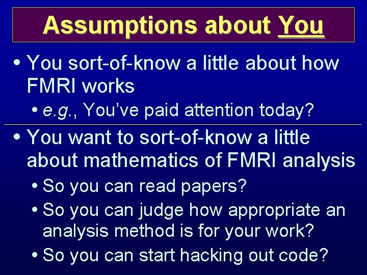
Assumptions about You • You sort-of-know a little about how FMRI works • e. g. , You’ve paid attention today? • You want to sort-of-know a little about mathematics of FMRI analysis • So you can read papers? • So you can judge how appropriate an analysis method is for your work? • So you can start hacking out code?

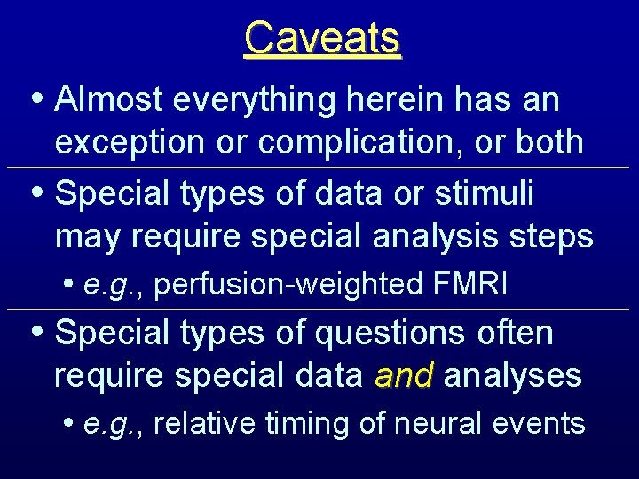
Caveats • Almost everything herein has an exception or complication, or both • Special types of data or stimuli may require special analysis steps • e. g. , perfusion-weighted FMRI • Special types of questions often require special data and analyses • e. g. , relative timing of neural events

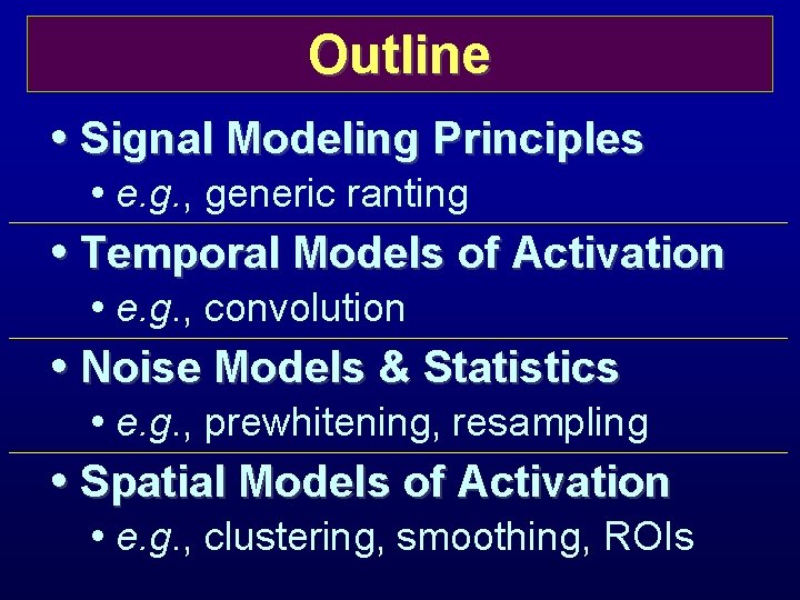
Outline • Signal Modeling Principles • e. g. , generic ranting • Temporal Models of Activation • e. g. , convolution • Noise Models & Statistics • e. g. , prewhitening, resampling • Spatial Models of Activation • e. g. , clustering, smoothing, ROIs

Signal Modeling Principles • Develop a mathematical model relating what we know (stimulus timing and image data) data to what we want to know (location, amount, timing, etc, of neural activity) activity • Given data, use this model to solve for unknown parameters in the neural activity (e. g. , when, where, how much, etc) • Then test for statistical significance

The Data • 10, 000. . 50, 000 image voxels inside brain (resolution 2 -3 mm) • 100. . 1000+ time points in each voxel (time step 2 s) • Also know timing of stimuli delivered to subject (etc) • Behavioral, physiological data? • Hopefully, some hypothesis

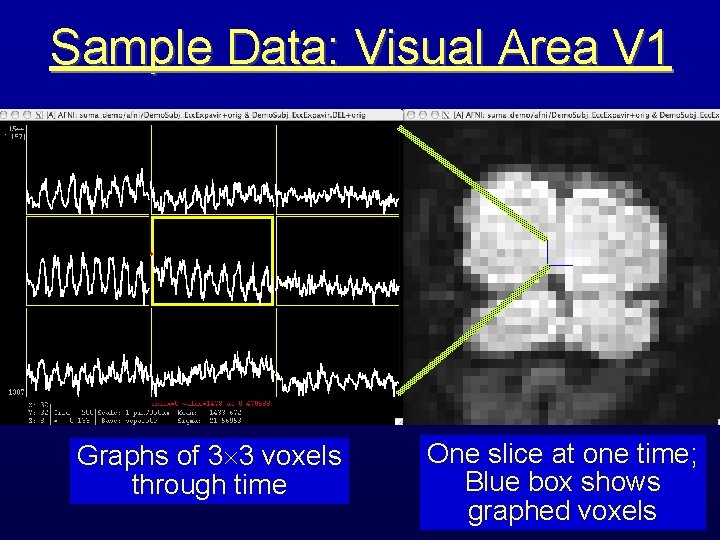
Sample Data: Visual Area V 1 Graphs of 3 3 voxels through time One slice at one time; Blue box shows graphed voxels

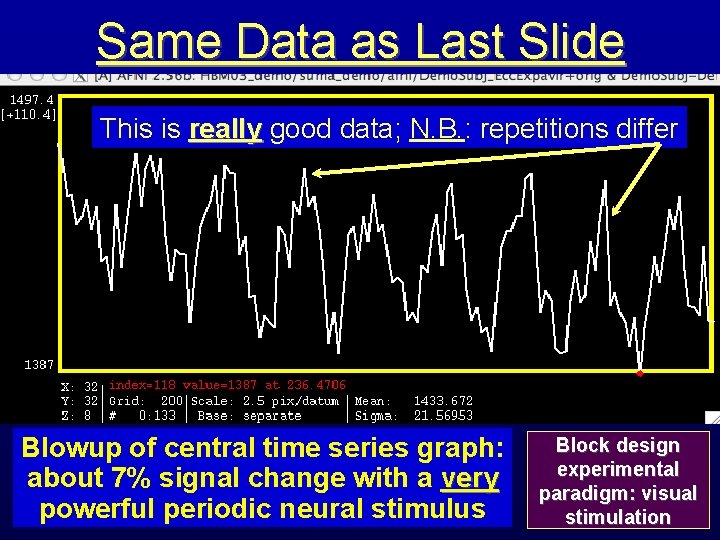
Same Data as Last Slide This is really good data; N. B. : repetitions differ Blowup of central time series graph: about 7% signal change with a very powerful periodic neural stimulus Block design experimental paradigm: visual stimulation

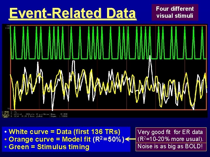
Event-Related Data • White curve = Data (first 136 TRs) • Orange curve = Model fit (R 2 = 50%) • Green = Stimulus timing Four different visual stimuli Very good fit for ER data (R 2=10 -20% more usual). Noise is as big as BOLD!

Why FMRI Analysis Is Hard • Don’t know true relation between neural “activity” and BOLD signal: • What is neural “activity”, anyway? • What is connection between “activity” and hemodynamics and MRI signal? • Noise in data is poorly characterized • In space and in time, and in origin • Noise amplitude BOLD signal • Can some of this noise be removed? • Makes both signal detection and statistical assessment hard

Why So Many Methods? • Different assumptions about activityto-MRI signal connection • Different assumptions about noise ( signal fluctuations of no interest) properties and statistics • Different experiments and questions • Result: Result Many “reasonable” FMRI analysis methods • Researchers must understand the tools!! (Models and software)

Fundamental Principles Underlying Most FMRI Analyses (esp. GLM): HRF Blobs • Hemodynamic Response Function • Convolution model for temporal relation between stimulus and response • Activation Blobs • Contiguous spatial regions whose voxel time series fit HRF model • e. g. , Reject isolated voxels even if HRF model fit is good there

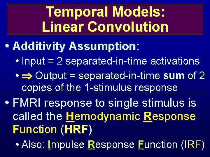
Temporal Models: Linear Convolution • Additivity Assumption: Assumption • Input = 2 separated-in-time activations • Output = separated-in-time sum of 2 copies of the 1 -stimulus response • FMRI response to single stimulus is called the Hemodynamic Response Function (HRF) HRF • Also: Impulse Response Function (IRF)

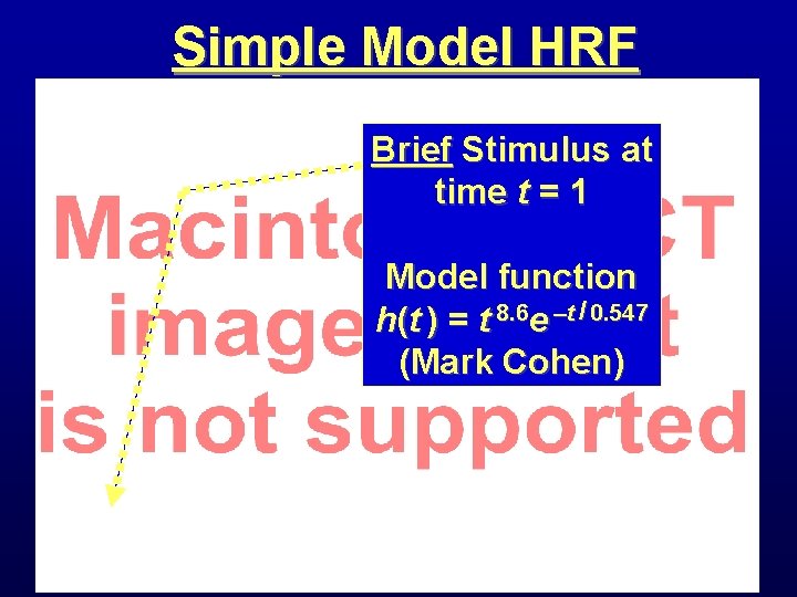
Simple Model HRF Brief Stimulus at time t = 1 Model function h(t ) = t 8. 6 e –t / 0. 547 (Mark Cohen)

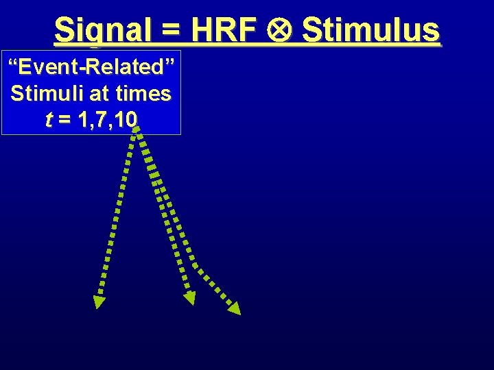
Signal = HRF Stimulus “Event-Related” Stimuli at times t = 1, 7, 10

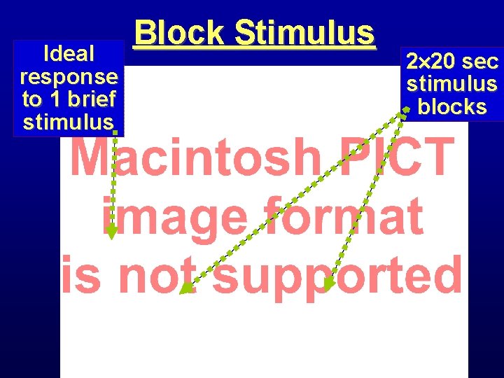
Ideal response to 1 brief stimulus Block Stimulus 2 20 sec stimulus blocks

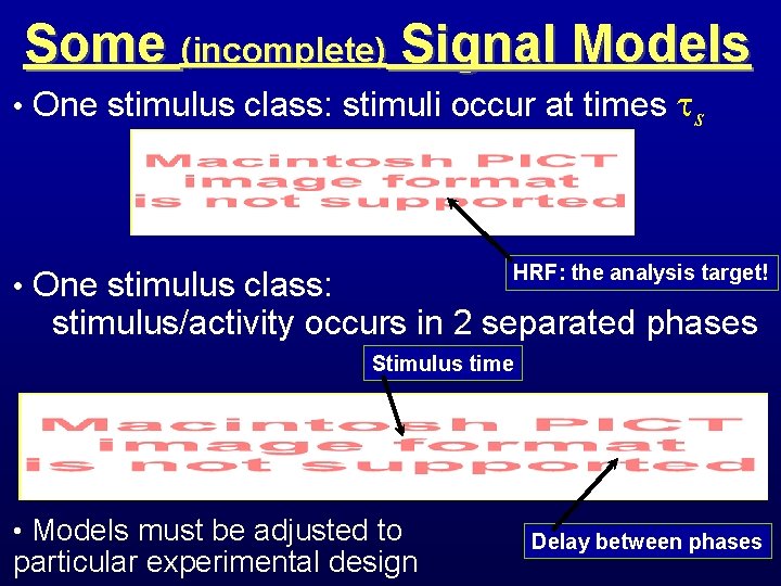
Some (incomplete) Signal Models • One stimulus class: stimuli occur at times s HRF: the analysis target! • One stimulus class: stimulus/activity occurs in 2 separated phases Stimulus time • Models must be adjusted to particular experimental design Delay between phases

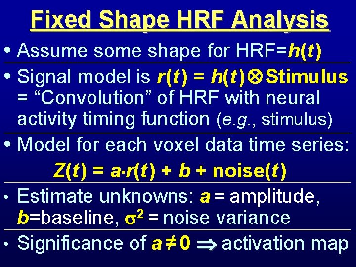
Fixed Shape HRF Analysis • Assume some shape for HRF=h(t ) • Signal model is r (t ) = h(t ) Stimulus = “Convolution” of HRF with neural activity timing function (e. g. , stimulus) • Model for each voxel data time series: Z(t ) = a r(t ) + b + noise(t ) • Estimate unknowns: a = amplitude, b=baseline, 2 = noise variance • Significance of a ≠ 0 activation map

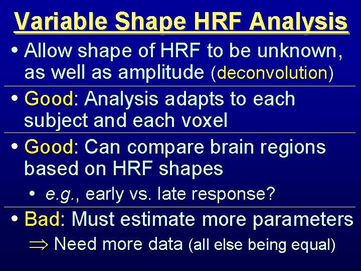
Variable Shape HRF Analysis • Allow shape of HRF to be unknown, as well as amplitude (deconvolution) • Good: Analysis adapts to each subject and each voxel • Good: Can compare brain regions based on HRF shapes • e. g. , early vs. late response? • Bad: Must estimate more parameters Þ Need more data (all else being equal)

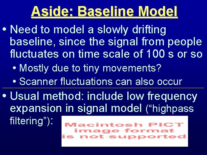
Aside: Baseline Model • Need to model a slowly drifting baseline, since the signal from people fluctuates on time scale of 100 s or so • Mostly due to tiny movements? • Scanner fluctuations can also occur • Usual method: include low frequency expansion in signal model (“highpass filtering”):

HRF Model Equations Simplest model: fixed shape Unknown = a [b & c fixed] Next simplest model: derivative allows for time shift Unknowns = a 0 and a 1 [b & c fixed] Expansion in a set of fixed basis functions { q(t )} (e. g. , Splines, sines, …); Unknowns = {wq}

Multiple Stimulus Classes • Need to calculate HRF (amplitude or amplitude+shape) separately for each class of stimulus • Novice FMRI researcher pitfall: try to use too many stimulus classes • Event-related FMRI: FMRI need 20+ events per stimulus class • Block design FMRI: FMRI need 10+ blocks per stimulus class

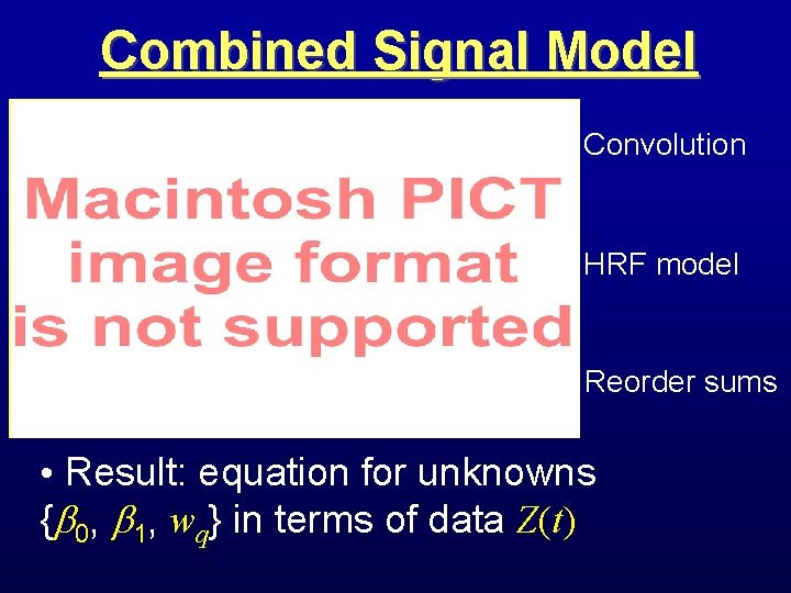
Combined Signal Model Convolution HRF model Reorder sums • Result: equation for unknowns { 0, 1, wq} in terms of data Z(t)

Matrix-Vector Formulation • Usually write equation in form: • In matrix-vector notation: Each column of R is a time series basis function, and each element of is its amplitude in z

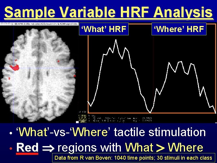
Sample Variable HRF Analysis ‘What’ HRF ‘Where’ HRF Where HRF What HRF ‘What’-vs-‘Where’ tactile stimulation • Red regions with What Where • Data from R van Boven: 1040 time points; 30 stimuli in each class

(Linear) Inverse Modeling • Instead of using stimulus timing to get HRF, could use an assumed HRF to get activity timing per voxel • Or could use an assumed spatial response (from a training/calibration run? ) to extract stimulus timing • e. g. , HBM 2006 Movie contest • Linear equations, but have swapped roles of unknowns & knowns

Noise Models & Statistics • Physiological “noise” • Heartbeat and respiration affect signal in complex ways • Subject head movement • After realignment, some effects remain • Low frequency drifts ( 0. 01 Hz) • Scanner glitches can produce gigantic ( 10 ) spikes in data

Physiological “Noise” • MRI signal changes due to nonneural physiology during scan • Can be approximately filtered out with external measurements • e. g. , respiratory bellows, pulse oximeter • Somewhat harder than it sounds, and is not commonly used (yet)

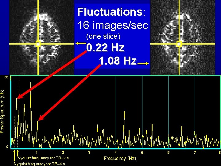
Fluctuations: 16 images/sec (one slice) 0. 22 Hz 1. 08 Hz

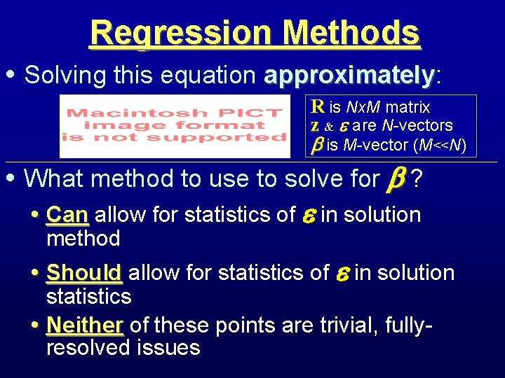
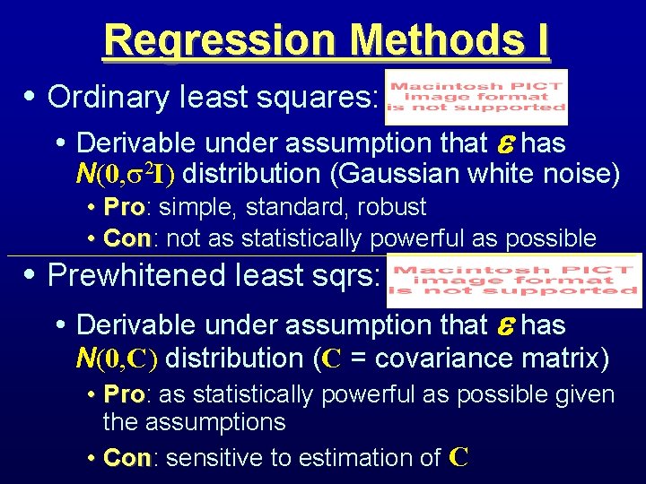
Regression Methods • Solving this equation approximately: approximately R is Nx. M matrix z & are N-vectors is M-vector (M<<N) • What method to use to solve for ? • Can allow for statistics of in solution method • Should allow for statistics of in solution statistics • Neither of these points are trivial, fullyresolved issues

Regression Methods I • Ordinary least squares: • Derivable under assumption that has N(0, 2 I) distribution (Gaussian white noise) • Pro: Pro simple, standard, robust • Con: Con not as statistically powerful as possible • Prewhitened least sqrs: • Derivable under assumption that has N(0, C) distribution (C = covariance matrix) • Pro: Pro as statistically powerful as possible given the assumptions • Con: Con sensitive to estimation of C

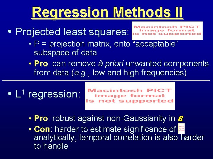
Regression Methods II • Projected least squares: • P = projection matrix, onto “acceptable” subspace of data • Pro: Pro can remove à priori unwanted components from data (e. g. , low and high frequencies) • L 1 regression: • Pro: Pro robust against non-Gaussianity in • Con: Con harder to estimate significance of analytically; temporal correlation is also harder to handle

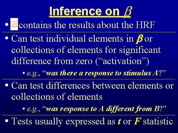
Inference on • contains the results about the HRF • Can test individual elements in or collections of elements for significant difference from zero (“activation”) • e. g. , “was there a response to stimulus A? ” • Can test differences between elements or collections of elements • e. g. , “was response to A different from B? ” • Tests usually expressed as t or F statistic

Estimating Serial Correlation • Can assume some model correlation structure; e. g. , AR(n) autoregressive models • Advantage is simplicity, not reality • Can try to estimate C directly • Possibly using neighboring voxels as well • Or smooth estimates of C (or some of the parameters in C) locally • Usually start with OLS to estimate and subtract “signal”, then estimate C from residuals

Adapting to Correlated Noise • Can adjust degrees-of-freedom in OLS estimates of parameters to approximate for correlation • Including correlation induced by projection via bandpass filters • If “properly” done, prewhitened LS will give full degrees-of-freedom with no semi-ad hoc adjustments required • Results can be sensitive to errors in C

Avoiding Some Assumptions • All statistical methods require assumptions about noise • Gaussianity, independence, … • Can use modern statistical resampling/permutation methods to reduce the number of assumptions • Very computationally intensive • Substituting number crunching for mathematical theory

Spatial Models of Activation • 10, 000. . 50, 000 image voxels in brain • Don’t really expect activation in a single voxel (usually) • Curse of multiple comparisons: • If have 10, 000 statistical tests to perform, and 5% give false positive, would have 500 voxels “activated” by pure noise — way too much! • Can group voxels together somehow to manage this curse

Spatial Grouping Methods • Smooth data in space before analysis • Average data across anatomicallyselected regions of interest ROI (before or after analysis) • Labor intensive (i. e. , send more postdocs) • Reject isolated small clusters of above-threshold voxels after analysis

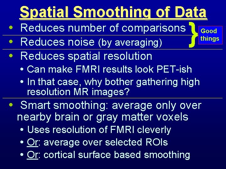
Spatial Smoothing of Data • Reduces number of comparisons • Reduces noise (by averaging) • Reduces spatial resolution } Good things • Can make FMRI results look PET-ish • In that case, why bother gathering high resolution MR images? • Smart smoothing: average only over nearby brain or gray matter voxels • Uses resolution of FMRI cleverly • Or: average over selected ROIs • Or: cortical surface based smoothing

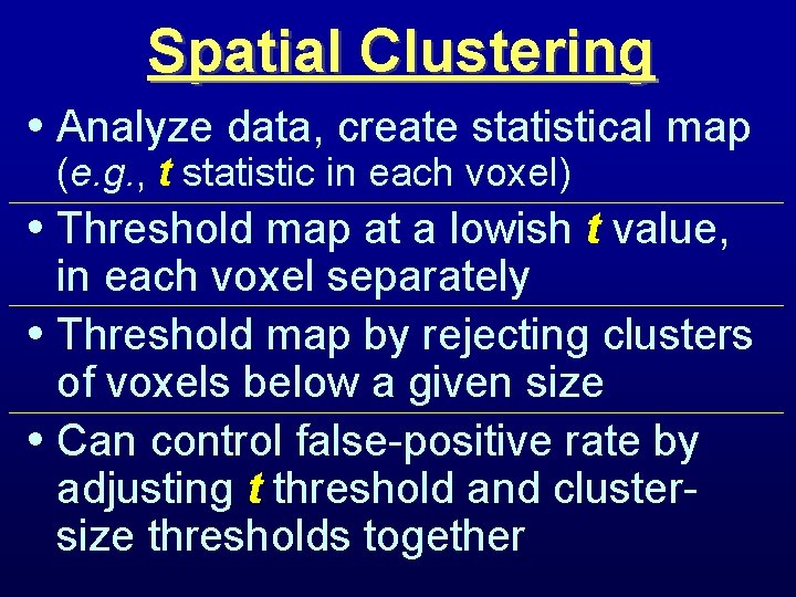
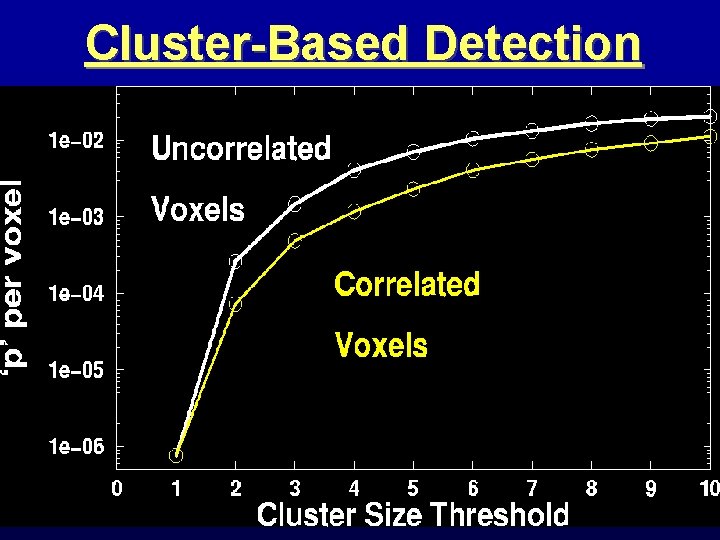
Spatial Clustering • Analyze data, create statistical map (e. g. , t statistic in each voxel) • Threshold map at a lowish t value, in each voxel separately • Threshold map by rejecting clusters of voxels below a given size • Can control false-positive rate by adjusting t threshold and clustersize thresholds together

Cluster-Based Detection

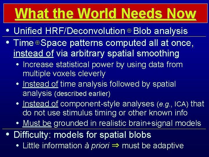
What the World Needs Now • Unified HRF/Deconvolution ⊕ Blob analysis • Time ⊕ Space patterns computed all at once, instead of via arbitrary spatial smoothing • Increase statistical power by using data from multiple voxels cleverly • Instead of time analysis followed by spatial analysis (described earlier) • Instead of component-style analyses (e. g. , ICA) that do not use stimulus timing or other known info • Must be grounded in realistic brain+signal models • Difficulty: models for spatial blobs • Little information à priori ⇒ must be adaptive

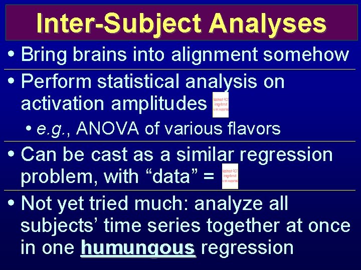
Inter-Subject Analyses • Bring brains into alignment somehow • Perform statistical analysis on activation amplitudes • e. g. , ANOVA of various flavors • Can be cast as a similar regression problem, with “data” = • Not yet tried much: analyze all subjects’ time series together at once in one humungous regression

Summary and Conclusion • FMRI data contain features that are about the same size as the BOLD signal and are poorly understood • Thus: Thus There are many “reasonable” ways to analyze FMRI data • Depending on the assumptions about the brain, the signal, and the noise • Conclusions: Conclusions Understand what you are doing & Look at your data • Or you will do something stupid

Finally … Thanks • The list of people I should thank is not quite endless … MM Klosek. JS Hyde. JR Binder. EA De. Yoe. SM Rao. EA Stein. A Jesmanowicz. MS Beauchamp. BD Ward. KM Donahue. PA Bandettini. AS Bloom. T Ross. M Huerta. ZS Saad. K Ropella. B Knutson. J Bobholz. G Chen. RM Birn. J Ratke. PSF Bellgowan. J Frost. K Bove-Bettis. R Doucette. RC Reynolds. PP Christidis. LR Frank. R Desimone. L Ungerleider. KR Hammett. DS Cohen. DA Jacobson. EC Wong. D Glen. Et alii … http: //afni. nimh. nih. gov/pub/tmp/ISMRM 2007/