Fluid Report Presentation Onur Erkal Korgun Koyunpnar Korhan

Fluid Report Presentation Onur Erkal Korgun Koyunpınar Korhan Türker Hakan Uzuner

Experiments Our fluid dynamics experiment is made up of two parts. 1) Determination of the velocity distribution of the air jet at different cross-sections and at different distances from the orifice to be able to calculate the discharge, momentum flux and kinetic energy flux. 2) Determination of the velocity distribution profiles of the air jet inside a pipe at different cross-sections which have different distances from the pipe inlet.

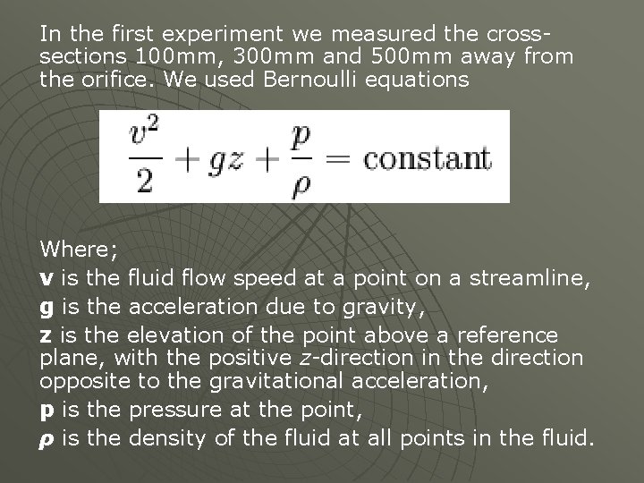
In the first experiment we measured the crosssections 100 mm, 300 mm and 500 mm away from the orifice. We used Bernoulli equations Where; v is the fluid flow speed at a point on a streamline, g is the acceleration due to gravity, z is the elevation of the point above a reference plane, with the positive z-direction in the direction opposite to the gravitational acceleration, p is the pressure at the point, ρ is the density of the fluid at all points in the fluid.

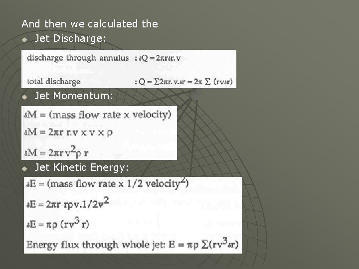
And then we calculated the u Jet Discharge: u Jet Momentum: u Jet Kinetic Energy:

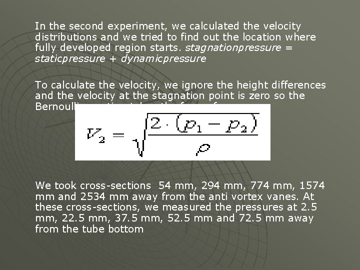
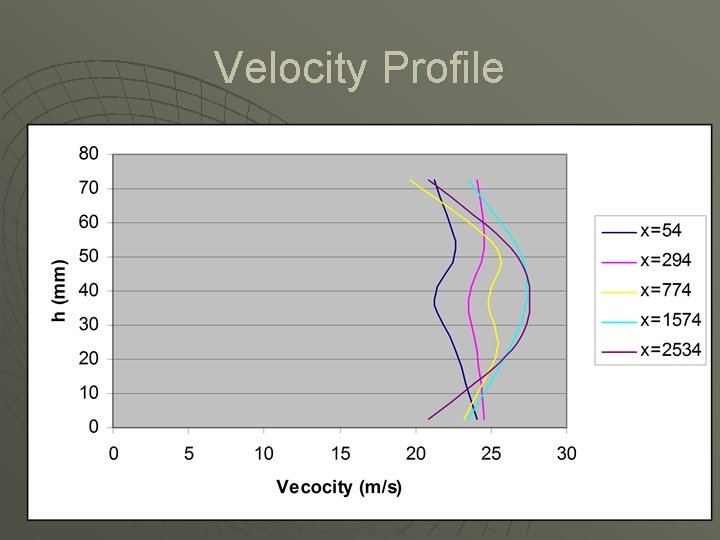
In the second experiment, we calculated the velocity distributions and we tried to find out the location where fully developed region starts. stagnationpressure = staticpressure + dynamicpressure To calculate the velocity, we ignore the height differences and the velocity at the stagnation point is zero so the Bernoulli equation takes the form of We took cross-sections 54 mm, 294 mm, 774 mm, 1574 mm and 2534 mm away from the anti vortex vanes. At these cross-sections, we measured the pressures at 2. 5 mm, 22. 5 mm, 37. 5 mm, 52. 5 mm and 72. 5 mm away from the tube bottom

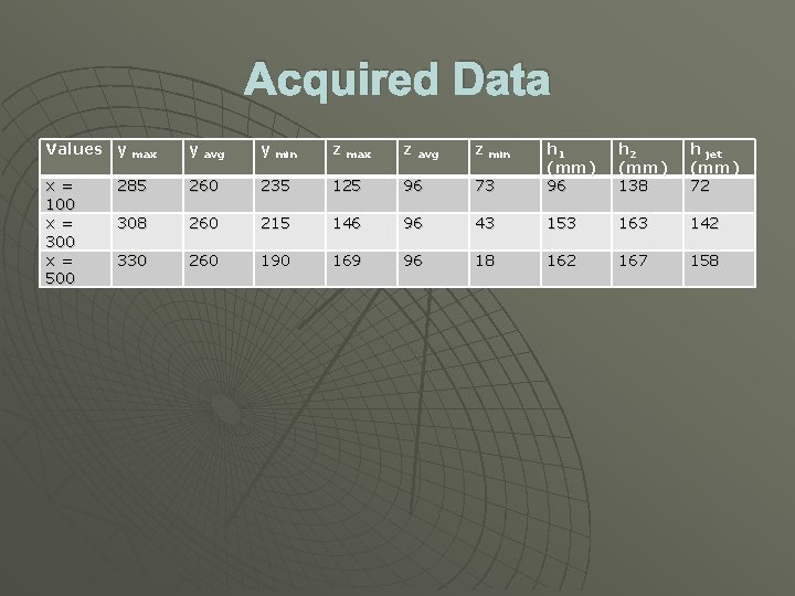
Results For this part of the experiment, the critical part was to calculate the h 1 and h 2 for different x values. Following is our recorded data from our experiment.

Acquired Data Values y max y avg y min z max z avg z min 73 h 1 (mm) 96 h 2 (mm) 138 h jet (mm) 72 x = 100 x = 300 x = 500 285 260 235 125 96 308 260 215 146 96 43 153 163 142 330 260 190 169 96 18 162 167 158

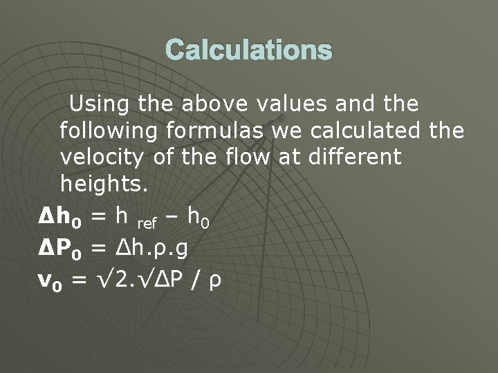
Calculations Using the above values and the following formulas we calculated the velocity of the flow at different heights. Δh 0 = h ref – h 0 ΔP 0 = Δh. ρ. g v 0 = √ 2. √ΔP / ρ

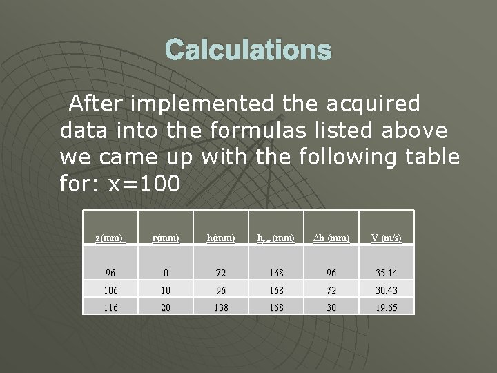
Calculations After implemented the acquired data into the formulas listed above we came up with the following table for: x=100 z(mm) r(mm) href (mm) ∆h (mm) V (m/s) 96 0 72 168 96 35. 14 106 10 96 168 72 30. 43 116 20 138 168 30 19. 65

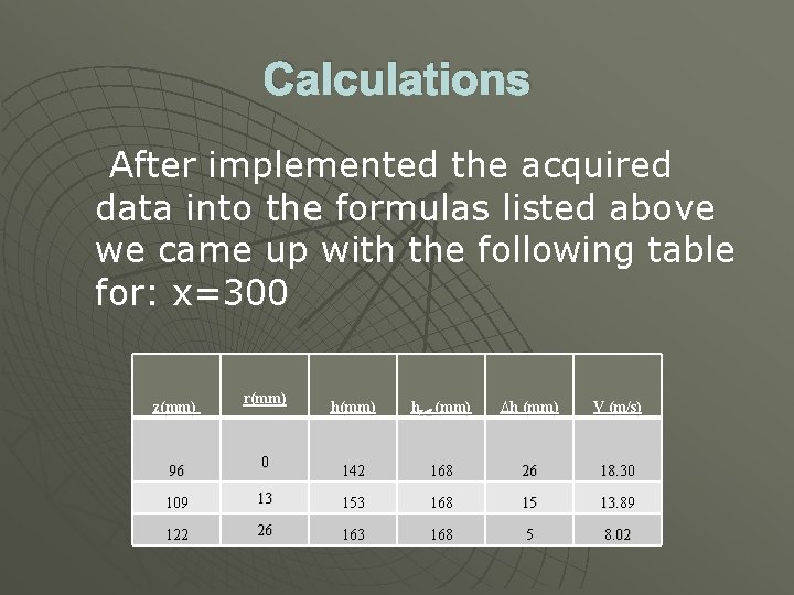
Calculations After implemented the acquired data into the formulas listed above we came up with the following table for: x=300 z(mm) 96 r(mm) 0 h(mm) href (mm) ∆h (mm) V (m/s) 142 168 26 18. 30 109 13 153 168 15 13. 89 122 26 163 168 5 8. 02

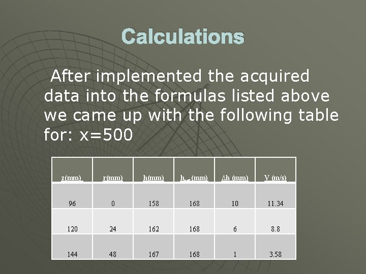
Calculations After implemented the acquired data into the formulas listed above we came up with the following table for: x=500 z(mm) r(mm) href (mm) ∆h (mm) V (m/s) 96 0 158 168 10 11. 34 120 24 162 168 6 8. 8 144 48 167 168 1 3. 58

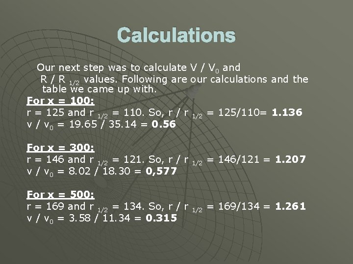
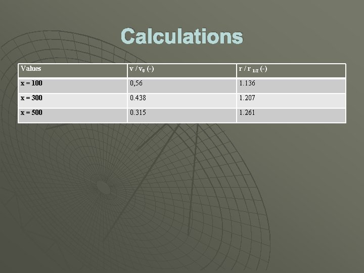
Calculations Our next step was to calculate V / V 0 and R / R 1/2 values. Following are our calculations and the table we came up with. For x = 100: r = 125 and r 1/2 = 110. So, r / r 1/2 = 125/110= 1. 136 v / v 0 = 19. 65 / 35. 14 = 0. 56 For x = 300: r = 146 and r 1/2 = 121. So, r / r 1/2 = 146/121 = 1. 207 v / v 0 = 8. 02 / 18. 30 = 0, 577 For x = 500: r = 169 and r 1/2 = 134. So, r / r 1/2 = 169/134 = 1. 261 v / v 0 = 3. 58 / 11. 34 = 0. 315

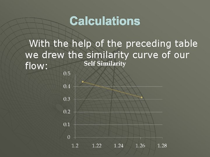
Calculations Values v / v 0 (-) r / r 1/2 (-) x = 100 0, 56 1. 136 x = 300 0. 438 1. 207 x = 500 0. 315 1. 261

Calculations With the help of the preceding table we drew the similarity curve of our flow:

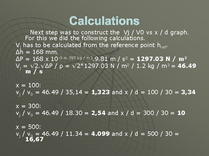
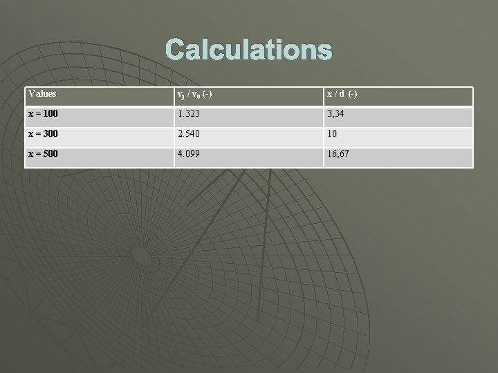
Calculations Next step was to construct the Vj / V 0 vs x / d graph. For this we did the following calculations. Vj has to be calculated from the reference point href. Δh = 168 mm. ΔP = 168 x 10 -3 m. 787 kg / m 3. 9. 81 m / s 2 = 1297. 03 N / m 2 Vj = √ 2. √ΔP / ρ = √ 2*1297. 03 N / m 2 / 1. 2 kg / m 3 = 46. 49 m/s x = 100: vj / v 0 = 46. 49 / 35, 14 = 1, 323 and x / d = 100 / 30 = 3, 34 x = 300: vj / v 0 = 46. 49 / 18. 30 = 2, 54 and x / d = 300 / 30 = 10 x = 500: vj / v 0 = 46. 49 / 11. 34 = 4. 099 and x / d = 500 / 30 = 16, 67

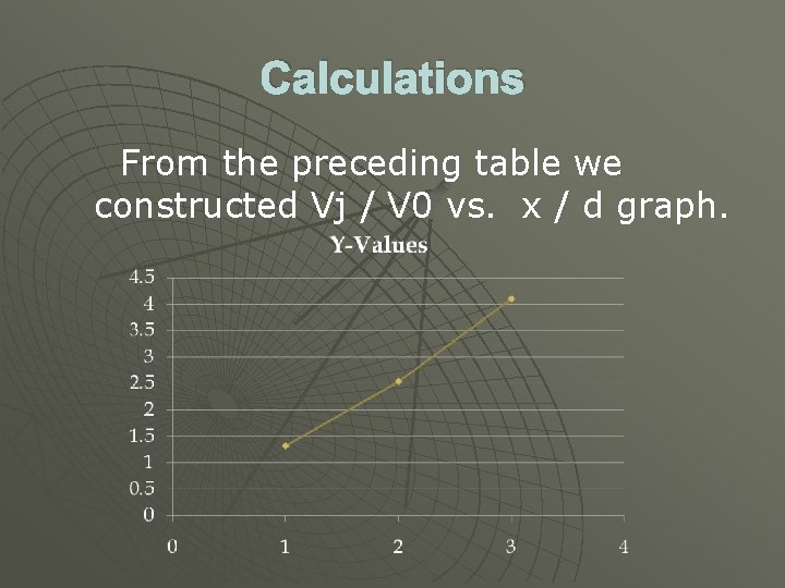
Calculations Values vj / v 0 (-) x / d (-) x = 100 1. 323 3, 34 x = 300 2. 540 10 x = 500 4. 099 16, 67

Calculations From the preceding table we constructed Vj / V 0 vs. x / d graph.

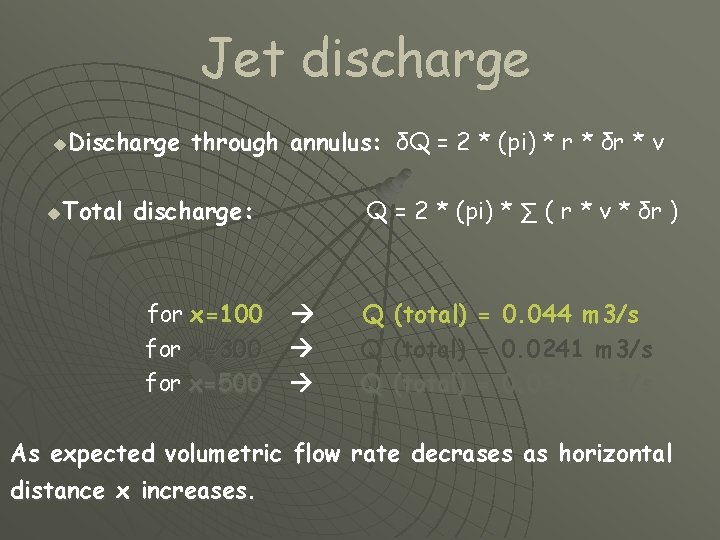
Jet discharge Discharge through annulus: δQ = 2 * (pi) * r * δr * v u Total discharge: Q = 2 * (pi) * ∑ ( r * v * δr ) u for x=100 for x=300 for x=500 Q Q Q (total) = = = 0. 044 m 3/s 0. 0241 m 3/s As expected volumetric flow rate decrases as horizontal distance x increases.

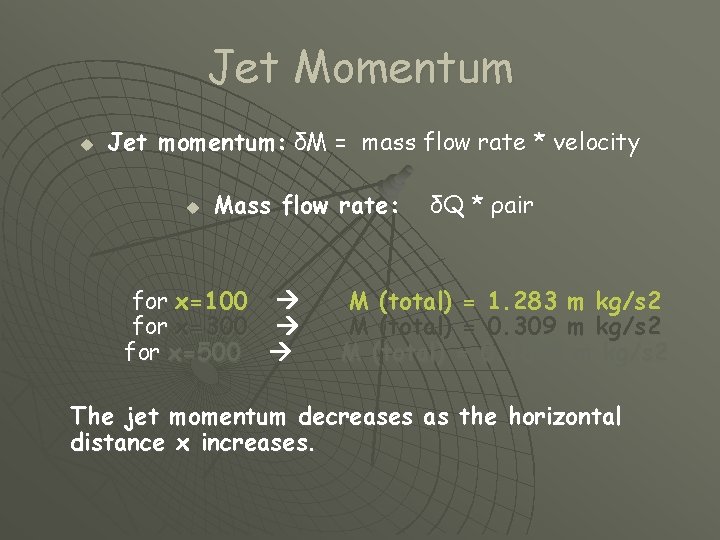
Jet Momentum u Jet momentum: δM = mass flow rate * velocity u Mass flow rate: for x=100 for x=300 for x=500 δQ * ρair M (total) = 1. 283 m kg/s 2 M (total) = 0. 309 m kg/s 2 M (total) = 0. 1878 m kg/s 2 The jet momentum decreases as the horizontal distance x increases.

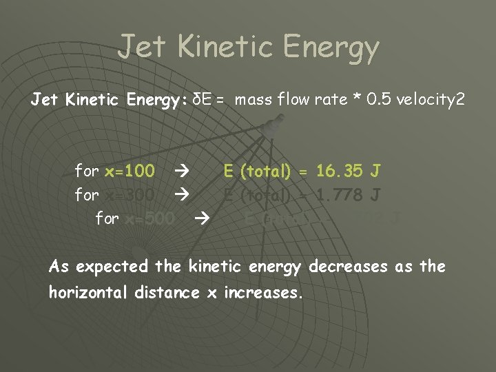
Jet Kinetic Energy: δE = mass flow rate * 0. 5 velocity 2 for x=100 E (total) = 16. 35 J for x=300 E (total) = 1. 778 J for x=500 E (total) = 0. 702 J As expected the kinetic energy decreases as the horizontal distance x increases.

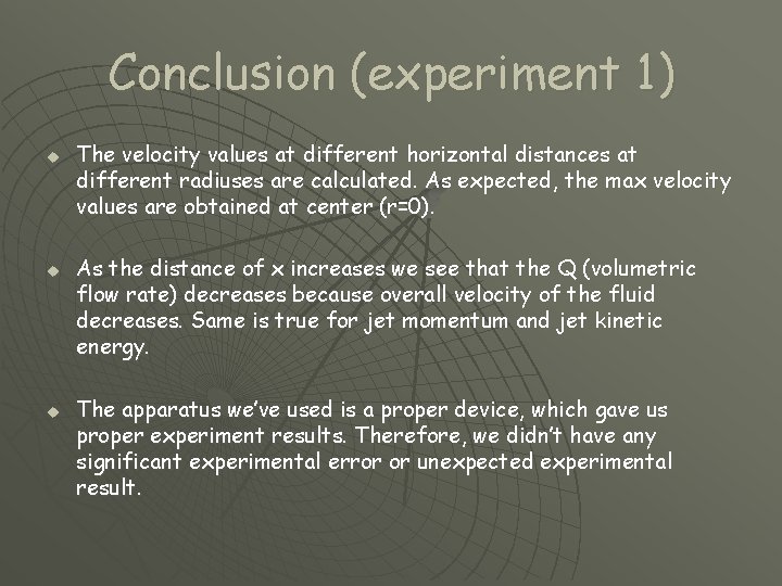
Conclusion (experiment 1) u u u The velocity values at different horizontal distances at different radiuses are calculated. As expected, the max velocity values are obtained at center (r=0). As the distance of x increases we see that the Q (volumetric flow rate) decreases because overall velocity of the fluid decreases. Same is true for jet momentum and jet kinetic energy. The apparatus we’ve used is a proper device, which gave us proper experiment results. Therefore, we didn’t have any significant experimental error or unexpected experimental result.

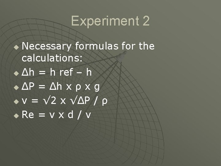
Experiment 2 Necessary formulas for the calculations: u Δh = h ref – h u ΔP = Δh x ρ x g u v = √ 2 x √ΔP / ρ u Re = v x d / ν u

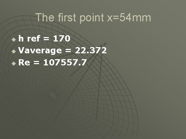
The first point x=54 mm h ref = 170 u Vaverage = 22. 372 u Re = 107557. 7 u

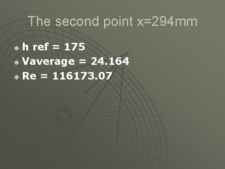
The second point x=294 mm h ref = 175 u Vaverage = 24. 164 u Re = 116173. 07 u

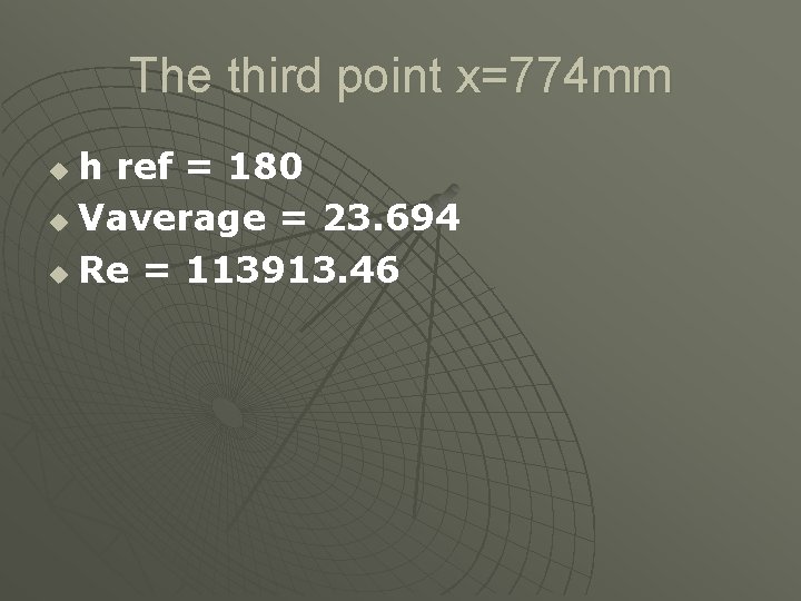
The third point x=774 mm h ref = 180 u Vaverage = 23. 694 u Re = 113913. 46 u

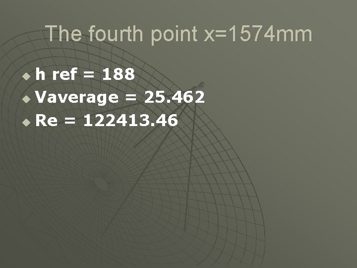
The fourth point x=1574 mm h ref = 188 u Vaverage = 25. 462 u Re = 122413. 46 u

The fifth point x=2534 mm h ref = 194 u Vaverage = 24. 418 u Re = 117394. 23 u

Velocity Profile

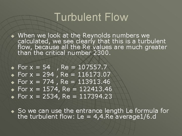
Turbulent Flow u u u u When we look at the Reynolds numbers we calculated, we see clearly that this is a turbulent flow, because all the Re values are much greater than the critical number 2300. For x = 54 , Re = 107557. 7 For x = 294 , Re = 116173. 07 For x = 774 , Re = 113913. 46 For x = 1574, Re = 122413. 46 For x = 2534, Re = 117394. 23 So we can use the entrance length Le formula for the turbulent flow: Le = 4, 4. Re average 1/6. d

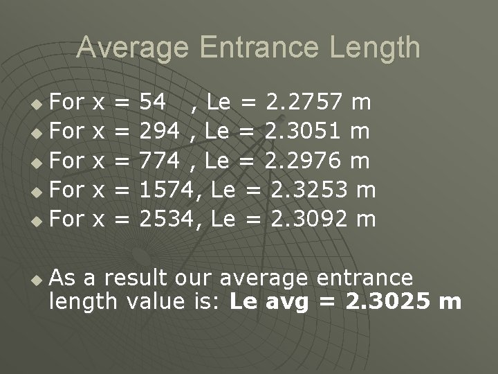
Average Entrance Length For x = 54 , Le = 2. 2757 m u For x = 294 , Le = 2. 3051 m u For x = 774 , Le = 2. 2976 m u For x = 1574, Le = 2. 3253 m u For x = 2534, Le = 2. 3092 m u u As a result our average entrance length value is: Le avg = 2. 3025 m

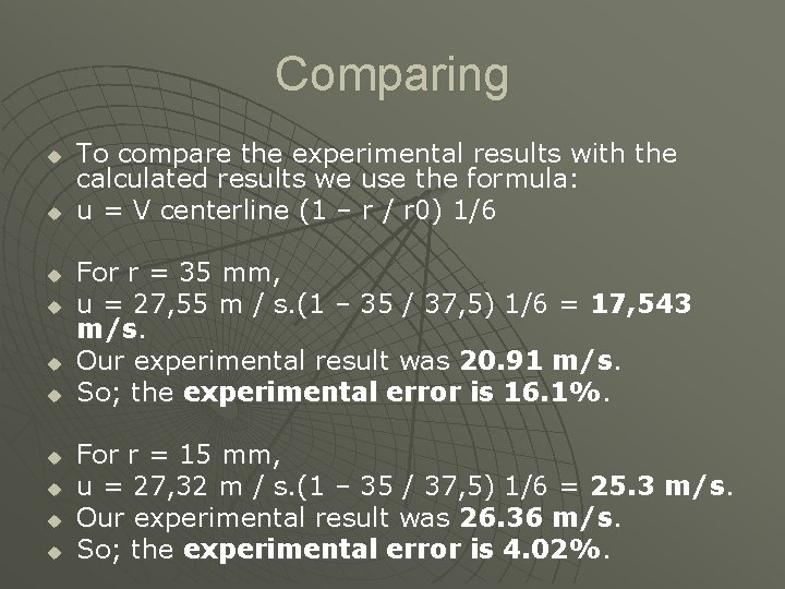
Comparing u u u u u To compare the experimental results with the calculated results we use the formula: u = V centerline (1 – r / r 0) 1/6 For r = 35 mm, u = 27, 55 m / s. (1 – 35 / 37, 5) 1/6 = 17, 543 m/s. Our experimental result was 20. 91 m/s. So; the experimental error is 16. 1%. For r = 15 mm, u = 27, 32 m / s. (1 – 35 / 37, 5) 1/6 = 25. 3 m/s. Our experimental result was 26. 36 m/s. So; the experimental error is 4. 02%.