Flow of mechanically incompressible but thermally expansible viscous

Flow of mechanically incompressible, but thermally expansible viscous fluids A. Mikelic, A. Fasano, A. Farina Montecatini, Sept. 9 - 17

LECTURE 1. Basic mathemathical modelling LECTURE 2. Mathematical problem LECTURE 3. Stability

Following standard mechanics arguments we have obteined:

We now write explicitly the equations governing the flow. 1. Energy equation where and recall the constraint

From definition and y = e –T s, we have

This term gives the classical

mechanical energy converted into heat by the internal friction

Remark 1. The coefficient in front of represents, from the physical point of view, the isobaric specific heat. The fluid we are modelling admits only the isobaric specific heat. Indeed any change of body's temperature implies a change in volume. Hence it is not possible to work with the isochoric specific heat cv

Remark 2. Experiments show that the variations of cp with respect to pressure are generally quite small. Hence we impose that cp (p, T) is constant with respect to the pressure field p. Thus we require b is of this form with TR reference temperature and b. R=b(TR )

As a consequence, from we have the following law for the density We will consider the linearized version, namely We however remark that, from the mathematical point of view such a Simplifcation is not crucial and it is consistent with the data reported in the experimental literature.

Remark 3. We remark that in the framework of the mechanical incompressibility assumption, the term is necessarily compensated by the mechanical work associated with dilation. Thus it does not appear in the energy balance. Indeed we have developed theory assuming that the constraint response does not dissipate energy.

Remark 4. Measuring cp we can reconstruct the Helmoltz free energy y. Indeed We have a method for “quantifying” y( T )

2. Momentum equation Next, we introduce the hydraulic head so that thus getting

Concerning the viscosity m we assume the. Vogel-Fulcher-Tamman's (VFT) formula In particular, m is monotonically decreasing with T. For more details we refer to [4], chapter 6. [4]. J. E. Shelby, Introduction to Glass Science and Technology, 2005.

3. Complete system

Non-Dimensionalization The scaling of model (1) has to be operated paying particular attention to the specific problem we are interested in. We are considering a gravity driven x 3 flow of melted glass through a Gi H nozzle in the early stage of a fiber n manufacturing process. The inlet and outlet temperature of R (x 3, f) the fluid are prescribed. In particular, Glat the fluid temperature on Gin is higher than the on Gout. 0 Gout

Concerning the temperature, we introduce so that Moreover we introduce also In the phenomena we are considering Typically is of order 10 -1. is small but not negligible.

The characteristic of the problem we are analyzing is that there exists a reference velocity VR. This makes our approach different from the ones presented in [5] and in [6] where there is no velocity scale defined by exterior conditions. The flow takes place in a nozzle of radius R and length H, with R/H=O (1). Hence we take H as length scale. Concerning the time scale we take t. R=H/VR [5]. Rajagopal, Ruzicka, Srinivasa, M 3 AS 1996. [6]. Gallavotti, Foundations of Fluid Dynamics, 2002

As the reference pressure PR we take the point of view that flows of glass or polymer melts are essentially dominated by viscous effects. Accordingly we set Notice that PR 0 as VR tends to 0 and, as a consequence p tends to the hydrostatic pressure. This is consistent with the fact that P “measures” the deviation of the pressure from the hydrostatic-one due to the fluid motion.

Summarizing, we have the following dimensionless quantities

Suppressing tildas to keep notation simple, model (1) rewrites

We now list the non-dimensional characteristic numbers appearing in the previous model • We may write • • •

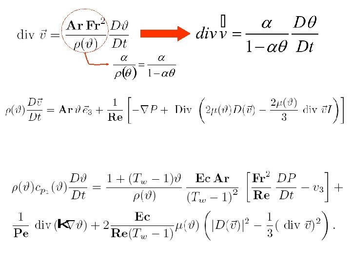
As mentioned, we are interested in studying vertical slow flows of very viscous heated fluids (molten glasses, polymer, etc. ) which are thermally dilatable. So, introducing the so-called expansivity coefficient (or thermal expansion coefficient) We will consider the mathematical system in the realistic situation in which the parameter a is small. Typically (e. g. for molten glass) In particular, as can be rewritten