FIXEDINCOME SECURITIES Chapter 12 Modeling the Yield Curve

FIXED-INCOME SECURITIES Chapter 12 Modeling the Yield Curve Dynamics

Outline • • • Motivation Interest Rate Trees Single-Factor Continuous-Time Models Multi-Factor Continuous-Time Models Arbitrage Models

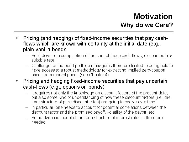
Motivation Why do we Care? • Pricing (and hedging) of fixed-income securities that pay cashflows which are known with certainty at the initial date (e. g. , plain vanilla bonds – Boils down to a computation of the sum of these cash-flows, discounted at a suitable rate – Challenge for the bond portfolio manager is therefore limited to being able to have access to a robust methodology for extracting implied zero-coupon prices from market prices (see Chapter 4) • Pricing and hedging fixed-income securities that pay uncertain cash-flows (e. g. , options on bonds) – It requires not only the knowledge on discount factors at the present date, but also some kind of understanding of how these discount factors (i. e. , the term structure of pure discount rates) are going to evolve over time – In particular, one needs to account for potential correlations between the discount factor and the promised payoff, volatility of the payoff, etc. – Some dynamic model of the term structure of interest rates is therefore needed

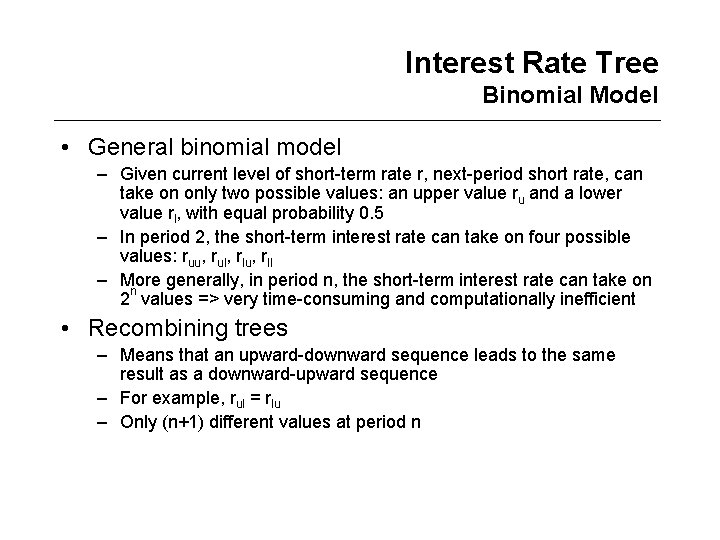
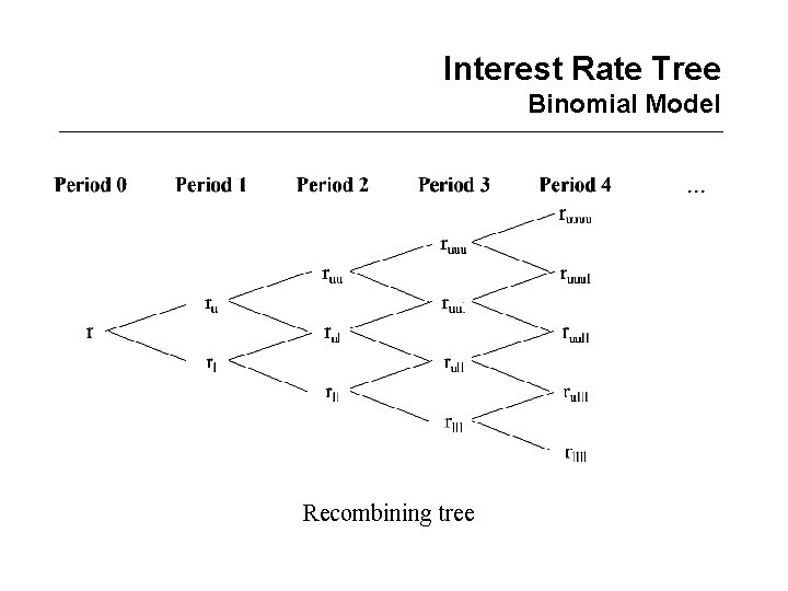
Interest Rate Tree Binomial Model • General binomial model – Given current level of short-term rate r, next-period short rate, can take on only two possible values: an upper value ru and a lower value rl, with equal probability 0. 5 – In period 2, the short-term interest rate can take on four possible values: ruu, rul, rlu, rll – More generally, in period n, the short-term interest rate can take on n 2 values => very time-consuming and computationally inefficient • Recombining trees – Means that an upward-downward sequence leads to the same result as a downward-upward sequence – For example, rul = rlu – Only (n+1) different values at period n

Interest Rate Tree Binomial Model Recombining tree

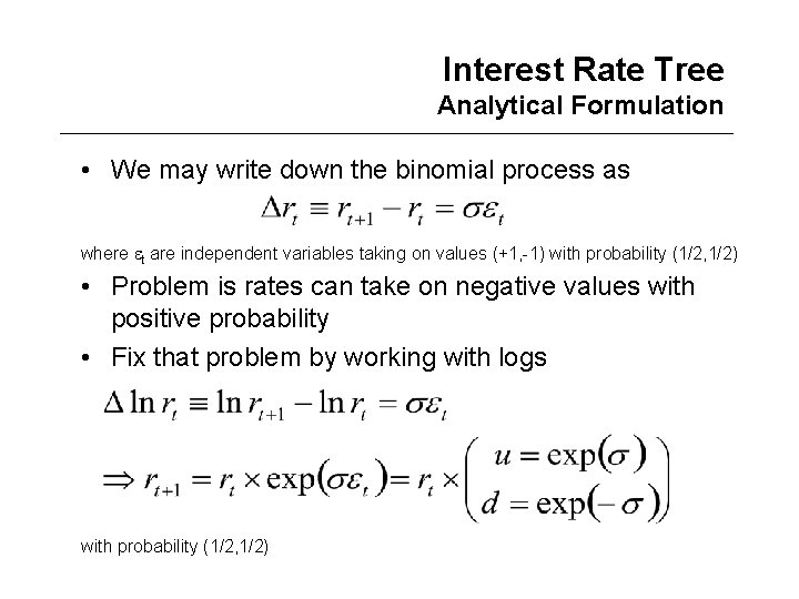
Interest Rate Tree Analytical Formulation • We may write down the binomial process as where t are independent variables taking on values (+1, -1) with probability (1/2, 1/2) • Problem is rates can take on negative values with positive probability • Fix that problem by working with logs with probability (1/2, 1/2)

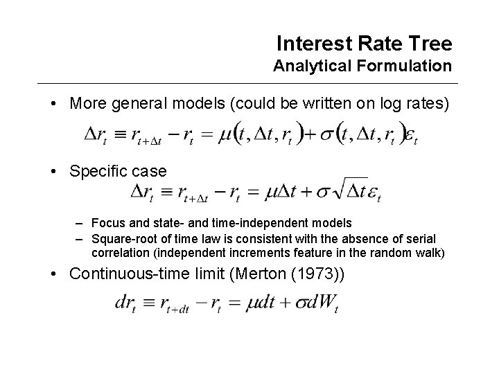
Interest Rate Tree Analytical Formulation • More general models (could be written on log rates) • Specific case – Focus and state- and time-independent models – Square-root of time law is consistent with the absence of serial correlation (independent increments feature in the random walk) • Continuous-time limit (Merton (1973))

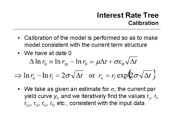
Interest Rate Tree Calibration • Calibration of the model is performed so as to make model consistent with the current term structure • We have at date 0 • We take as given an estimate for , the current par yield curve yt, and we iteratively find the values ru, rl, ruu, rul, rlu, rll, etc. , consistent with the input data

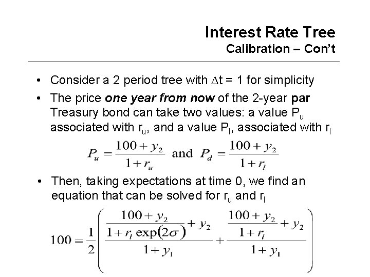
Interest Rate Tree Calibration – Con’t • Consider a 2 period tree with t = 1 for simplicity • The price one year from now of the 2 -year par Treasury bond can take two values: a value Pu associated with ru, and a value Pl, associated with rl • Then, taking expectations at time 0, we find an equation that can be solved for ru and rl

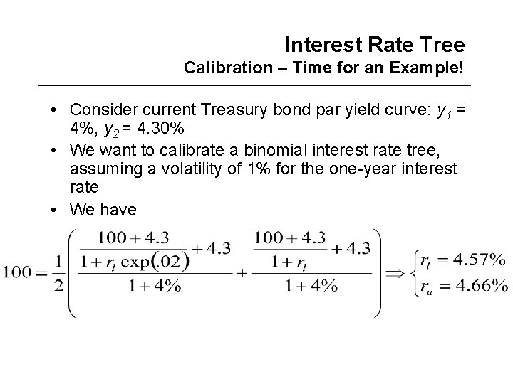
Interest Rate Tree Calibration – Time for an Example! • Consider current Treasury bond par yield curve: y 1 = 4%, y 2 = 4. 30% • We want to calibrate a binomial interest rate tree, assuming a volatility of 1% for the one-year interest rate • We have

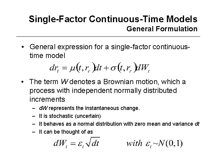
Single-Factor Continuous-Time Models General Formulation • General expression for a single-factor continuoustime model • The term W denotes a Brownian motion, which a process with independent normally distributed increments – – d. W represents the instantaneous change. It is stochastic (uncertain) It behaves as a normal distribution with zero mean and variance dt It can be thought of as

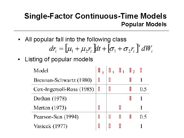
Single-Factor Continuous-Time Models Popular Models • All popular fall into the following class • Listing of popular models

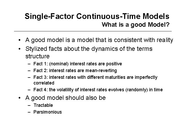
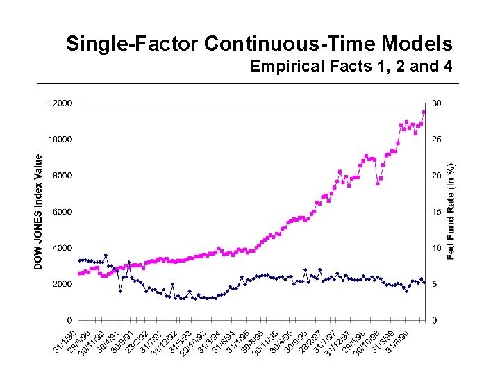
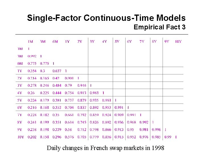
Single-Factor Continuous-Time Models What is a good Model? • A good model is a model that is consistent with reality • Stylized facts about the dynamics of the terms structure – Fact 1: (nominal) interest rates are positive – Fact 2: interest rates are mean-reverting – Fact 3: interest rates with different maturities are imperfectly correlated – Fact 4: the volatility of interest rates evolves (randomly) in time • A good model should also be – Tractable – Parsimonious

Single-Factor Continuous-Time Models Empirical Facts 1, 2 and 4

Single-Factor Continuous-Time Models Empirical Fact 3 Daily changes in French swap markets in 1998

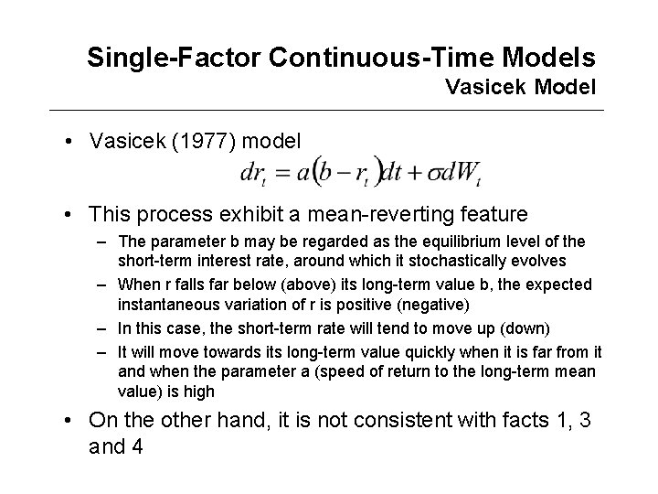
Single-Factor Continuous-Time Models Vasicek Model • Vasicek (1977) model • This process exhibit a mean-reverting feature – The parameter b may be regarded as the equilibrium level of the short-term interest rate, around which it stochastically evolves – When r falls far below (above) its long-term value b, the expected instantaneous variation of r is positive (negative) – In this case, the short-term rate will tend to move up (down) – It will move towards its long-term value quickly when it is far from it and when the parameter a (speed of return to the long-term mean value) is high • On the other hand, it is not consistent with facts 1, 3 and 4

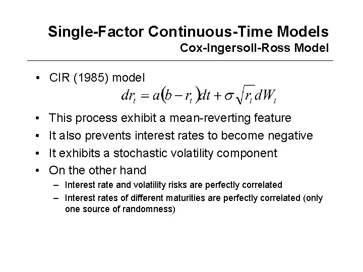
Single-Factor Continuous-Time Models Cox-Ingersoll-Ross Model • CIR (1985) model • • This process exhibit a mean-reverting feature It also prevents interest rates to become negative It exhibits a stochastic volatility component On the other hand – Interest rate and volatility risks are perfectly correlated – Interest rates of different maturities are perfectly correlated (only one source of randomness)

Multi-Factor Continuous-Time Models Some Popular Models • Fong and Vasicek (1991) model – Fong and Vasicek (1991) take the short rate and its volatility as two state variables – Variance of the short-rate changes is a key element in the pricing of fixed-income securities, in particular interest rates derivatives • Longstaff and Schwartz (1992) model – Longstaff and Schwartz (1992) use the same two state variables, but with a different specification – Allows them to get closed-form solution for the price of a discount bond a call option on a discount bond • Chen (1996) and Balduzzi et al. (1996) models – Chen (1996) and Balduzzi et al. (1996) suggest the use of a threefactor model by adding the short-term average of the short rate – These three state variables can be assimilated to the three factors which can be empirically obtained though a PCA of the term structure dynamics

Arbitrage Models Calibration of Continuous-Time Factor Models • In practice, single or multi-factor models are calibrated in such a way that the models' parameters are obtained as solutions to a minimization program of the difference (i. e. , the squared spread) between market prices of reference bonds and theoretical values generated from the model • This is the analogue of the calibration of an interest rate tree • Then the model is used to price interest rates derivatives (see Chapters 14 and 15) • The difference between the derived yield curve and the observed curve, even though minimized, can not be entirely eliminated

Arbitrage Models Some Popular Models • These models are built to be consistent with currently observed bond prices, which makes them popular among practitioners • First example is Ho and Lee (1986) – Discrete-time binomial setting – Discount bond prices are driven by a single source of uncertainty • Heath, Jarrow and Morton (1990 ab, 1992) have generalized this approach by allowing discount bonds prices to be driven by a multi-dimensional uncertainty in a continuous-time framework • Markovian versions of the HJM model are often used – Translate into recombining trees in discrete-time – Can be implemented without too much numerical complexity