Fixed v RandomEffects Fixed and Random Effects 1
- Slides: 22

Fixed- v. Random-Effects

Fixed and Random Effects 1 All conditions of interest – Fixed. Sample of interest – Random. Both fixed and random-effects meta-analyses attribute some observed variance to sampling error. For clear statements about fixed vs. random: Viechtbauer W: Conducting meta-analysis in R with the metafor package. Journal of Statistical Software 2010, 36(3): 1 -48. Bonett DG: Meta-analytic interval estimation for Pearson correlations. Psychological Methods 2008, 13: 173 -189.

Fixed & Random 2 The residual variance after accounting for sampling error (and maybe other variables) is called random-effects variance. Some people say ‘between studies variance. ’ REVC is the random-effects variance component. Hedges calls the REVC tau-squared - τ2. Hunter & Schmidt talk about SDrho (square root of same). Both refer to REVC Problem is that our interest is random – want to generalize beyond current sample, but our observations (studies) are not a random sample. Data are problematic for the kind of inference we want to make.

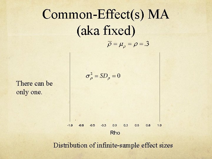
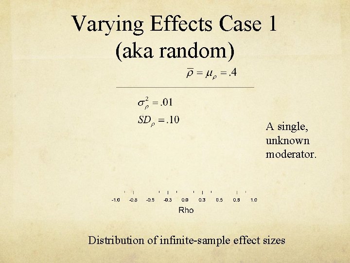
Fixed vs. Random 3 In the literature, fixed vs random is confused with common vs. varying effects meta-analysis. Common effect MA – only a single population parameter Varying effects MA – parameter has a distribution (typically assumed to be Normal) I will usually say ‘random effects’ when I mean to say ‘varying effects’. Mixed Model Fixed Moderators (aka covariates) Remaining (random-effects) variance

Common-Effect(s) MA (aka fixed) There can be only one. Distribution of infinite-sample effect sizes

Varying Effects Case 1 (aka random) A single, unknown moderator. Distribution of infinite-sample effect sizes

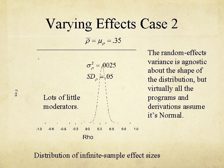
Varying Effects Case 2 Lots of little moderators. The random-effects variance is agnostic about the shape of the distribution, but virtually all the programs and derivations assume it’s Normal. Distribution of infinite-sample effect sizes

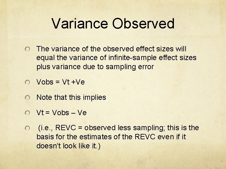
Variance Observed The variance of the observed effect sizes will equal the variance of infinite-sample effect sizes plus variance due to sampling error Vobs = Vt +Ve Note that this implies Vt = Vobs – Ve (i. e. , REVC = observed less sampling; this is the basis for the estimates of the REVC even if it doesn’t look like it. )

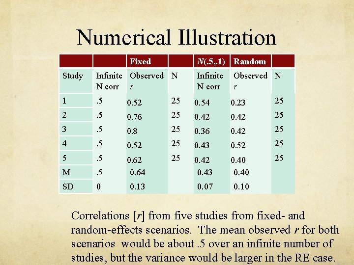
Numerical Illustration Fixed N(. 5, . 1) Random Study Infinite Observed N N corr r 1 . 5 0. 52 25 0. 54 0. 23 25 2 . 5 0. 76 25 0. 42 25 3 . 5 0. 8 25 0. 36 0. 42 25 4 . 5 0. 52 25 0. 43 0. 52 25 5 . 5 25 . 5 0. 42 0. 43 0. 40 25 M 0. 62 0. 64 SD 0 0. 13 0. 07 0. 10 Correlations [r] from five studies from fixed- and random-effects scenarios. The mean observed r for both scenarios would be about. 5 over an infinite number of studies, but the variance would be larger in the RE case.

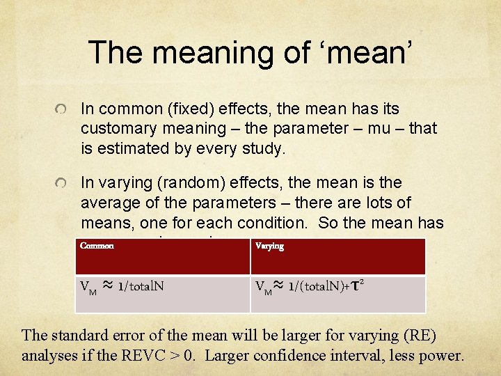
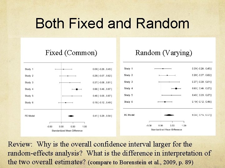
The meaning of ‘mean’ In common (fixed) effects, the mean has its customary meaning – the parameter – mu – that is estimated by every study. In varying (random) effects, the mean is the average of the parameters – there are lots of means, one for each condition. So the mean has an unusual meaning. Varying Common VM ≈ 1/total. N VM≈ 1/(total. N)+τ2 The standard error of the mean will be larger for varying (RE) analyses if the REVC > 0. Larger confidence interval, less power.

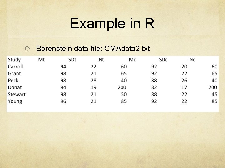
Example in R Borenstein data file: CMAdata 2. txt

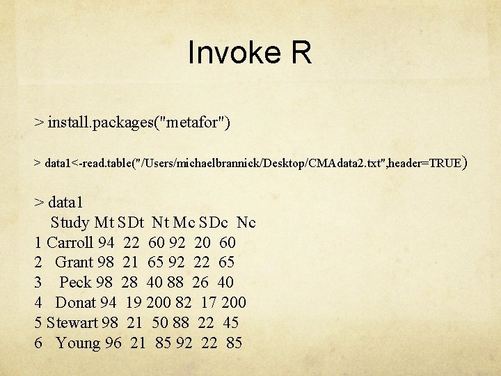
Invoke R > install. packages("metafor") > data 1<-read. table("/Users/michaelbrannick/Desktop/CMAdata 2. txt", header=TRUE ) > data 1 Study Mt SDt Nt Mc SDc Nc 1 Carroll 94 22 60 92 20 60 2 Grant 98 21 65 92 22 65 3 Peck 98 28 40 88 26 40 4 Donat 94 19 200 82 17 200 5 Stewart 98 21 50 88 22 45 6 Young 96 21 85 92 22 85

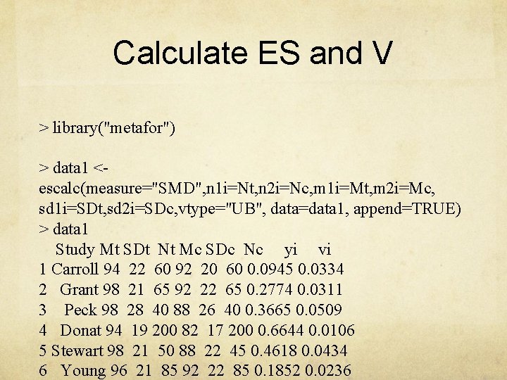
Calculate ES and V > library("metafor") > data 1 <- escalc(measure="SMD", n 1 i=Nt, n 2 i=Nc, m 1 i=Mt, m 2 i=Mc, sd 1 i=SDt, sd 2 i=SDc, vtype="UB", data=data 1, append=TRUE) > data 1 Study Mt SDt Nt Mc SDc Nc yi vi 1 Carroll 94 22 60 92 20 60 0. 0945 0. 0334 2 Grant 98 21 65 92 22 65 0. 2774 0. 0311 3 Peck 98 28 40 88 26 40 0. 3665 0. 0509 4 Donat 94 19 200 82 17 200 0. 6644 0. 0106 5 Stewart 98 21 50 88 22 45 0. 4618 0. 0434 6 Young 96 21 85 92 22 85 0. 1852 0. 0236

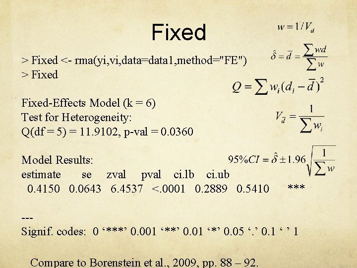
Fixed > Fixed <- rma(yi, vi, data=data 1, method="FE") > Fixed-Effects Model (k = 6) Test for Heterogeneity: Q(df = 5) = 11. 9102, p-val = 0. 0360 Model Results: estimate se zval pval ci. lb ci. ub 0. 4150 0. 0643 6. 4537 <. 0001 0. 2889 0. 5410 *** --Signif. codes: 0 ‘***’ 0. 001 ‘**’ 0. 01 ‘*’ 0. 05 ‘. ’ 0. 1 ‘ ’ 1 Compare to Borenstein et al. , 2009, pp. 88 – 92.

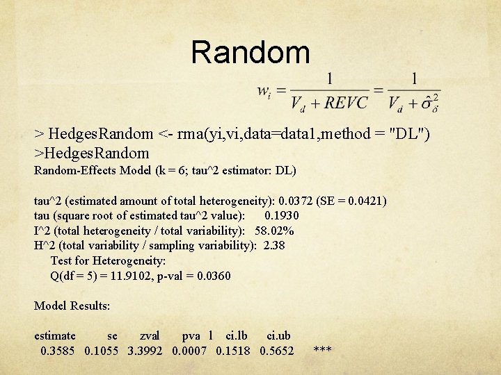
Random > Hedges. Random <- rma(yi, vi, data=data 1, method = "DL") >Hedges. Random-Effects Model (k = 6; tau^2 estimator: DL) tau^2 (estimated amount of total heterogeneity): 0. 0372 (SE = 0. 0421) tau (square root of estimated tau^2 value): 0. 1930 I^2 (total heterogeneity / total variability): 58. 02% H^2 (total variability / sampling variability): 2. 38 Test for Heterogeneity: Q(df = 5) = 11. 9102, p-val = 0. 0360 Model Results: estimate se zval pva l ci. lb ci. ub 0. 3585 0. 1055 3. 3992 0. 0007 0. 1518 0. 5652 ***

Both Fixed and Random Fixed (Common) Random (Varying) Review: Why is the overall confidence interval larger for the random-effects analysis? What is the difference in interpretation of the two overall estimates? (compare to Borenstein et al. , 2009, p. 89)

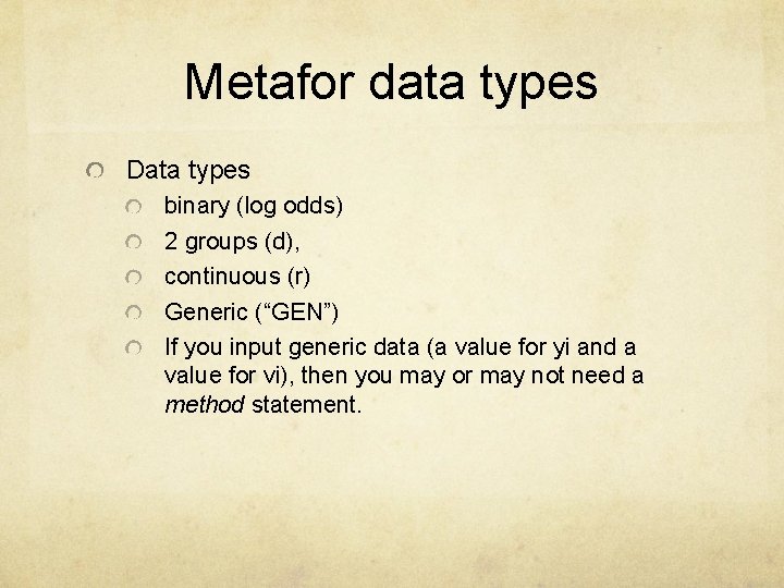
Metafor data types Data types binary (log odds) 2 groups (d), continuous (r) Generic (“GEN”) If you input generic data (a value for yi and a value for vi), then you may or may not need a method statement.

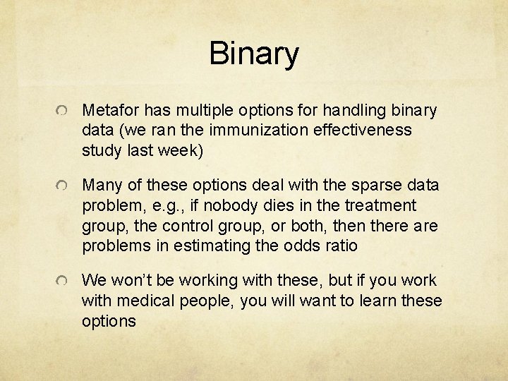
Binary Metafor has multiple options for handling binary data (we ran the immunization effectiveness study last week) Many of these options deal with the sparse data problem, e. g. , if nobody dies in the treatment group, the control group, or both, then there are problems in estimating the odds ratio We won’t be working with these, but if you work with medical people, you will want to learn these options

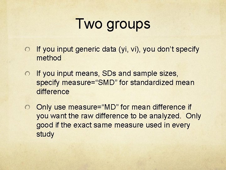
Two groups If you input generic data (yi, vi), you don’t specify method If you input means, SDs and sample sizes, specify measure=“SMD” for standardized mean difference Only use measure=“MD” for mean difference if you want the raw difference to be analyzed. Only good if the exact same measure used in every study

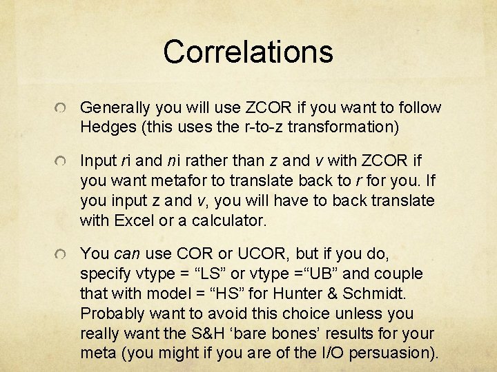
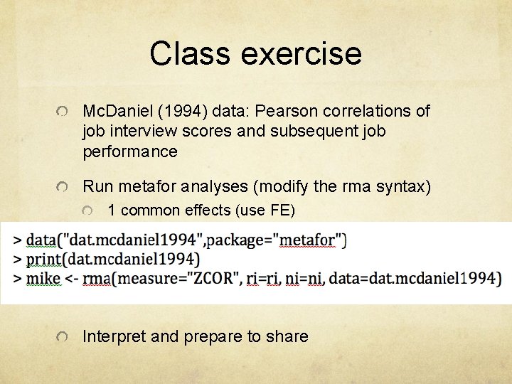
Correlations Generally you will use ZCOR if you want to follow Hedges (this uses the r-to-z transformation) Input ri and ni rather than z and v with ZCOR if you want metafor to translate back to r for you. If you input z and v, you will have to back translate with Excel or a calculator. You can use COR or UCOR, but if you do, specify vtype = “LS” or vtype =“UB” and couple that with model = “HS” for Hunter & Schmidt. Probably want to avoid this choice unless you really want the S&H ‘bare bones’ results for your meta (you might if you are of the I/O persuasion).

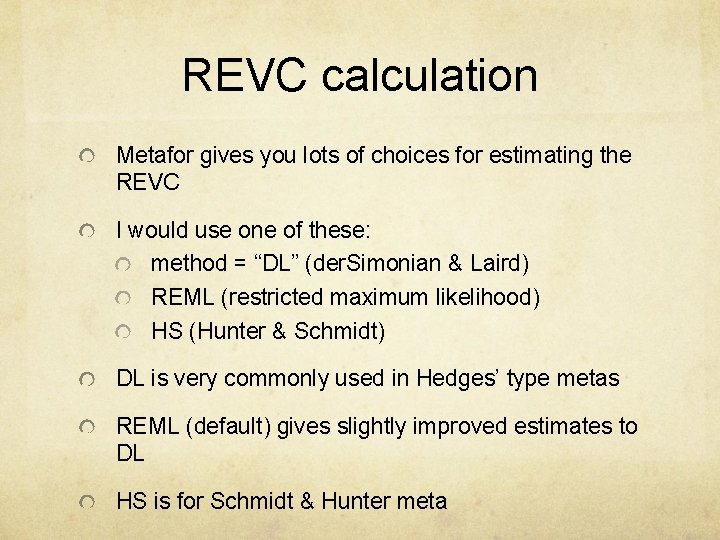
REVC calculation Metafor gives you lots of choices for estimating the REVC I would use one of these: method = “DL” (der. Simonian & Laird) REML (restricted maximum likelihood) HS (Hunter & Schmidt) DL is very commonly used in Hedges’ type metas REML (default) gives slightly improved estimates to DL HS is for Schmidt & Hunter meta

Class exercise Mc. Daniel (1994) data: Pearson correlations of job interview scores and subsequent job performance Run metafor analyses (modify the rma syntax) 1 common effects (use FE) 1 random effects (use DL) Interpret and prepare to share