Fixed and Random Effects Theory of Analysis of

Fixed and Random Effects

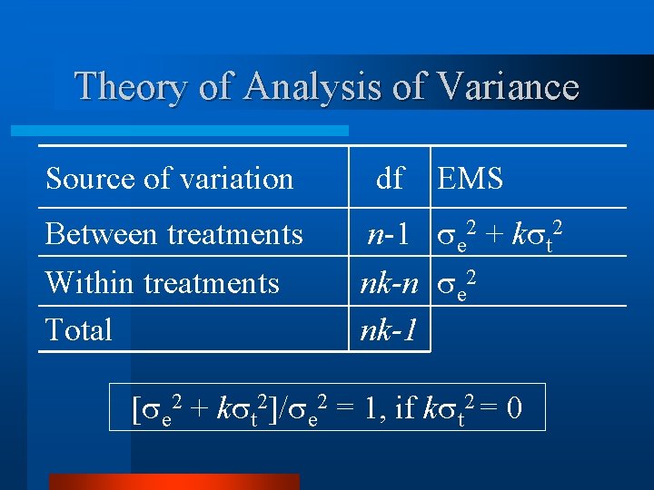
Theory of Analysis of Variance Source of variation df EMS Between treatments n-1 e 2 + k t 2 Within treatments Total nk-n e 2 nk-1 [ e 2 + k t 2]/ e 2 = 1, if k t 2 = 0

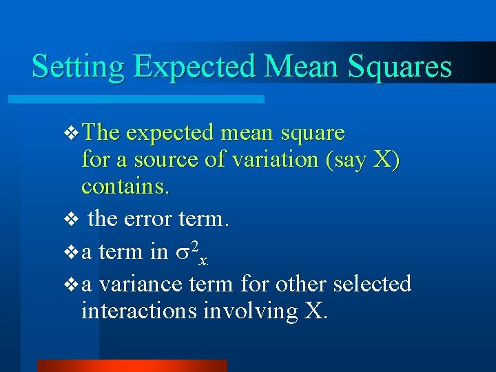
Setting Expected Mean Squares v The expected mean square for a source of variation (say X) contains. v the error term. v a term in 2 x. v a variance term for other selected interactions involving X.

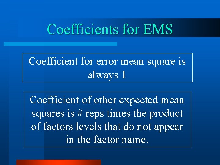
Coefficients for EMS Coefficient for error mean square is always 1 Coefficient of other expected mean squares is # reps times the product of factors levels that do not appear in the factor name.

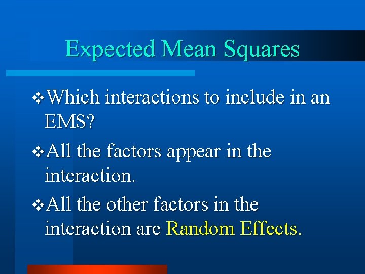
Expected Mean Squares v. Which interactions to include in an EMS? v. All the factors appear in the interaction. v. All the other factors in the interaction are Random Effects.

Pooling Sums of Squares

Multiple Comparisons

Multiple Comparisons v. Multiple Range Tests: Øt-tests and LSD’s; ØTukey’s and Duncan’s. v. Orthogonal Contrasts.

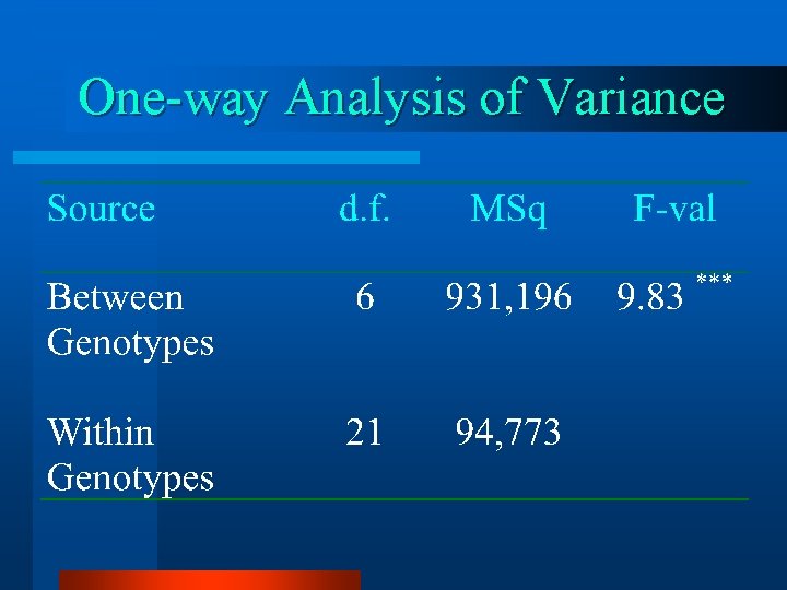
One-way Analysis of Variance

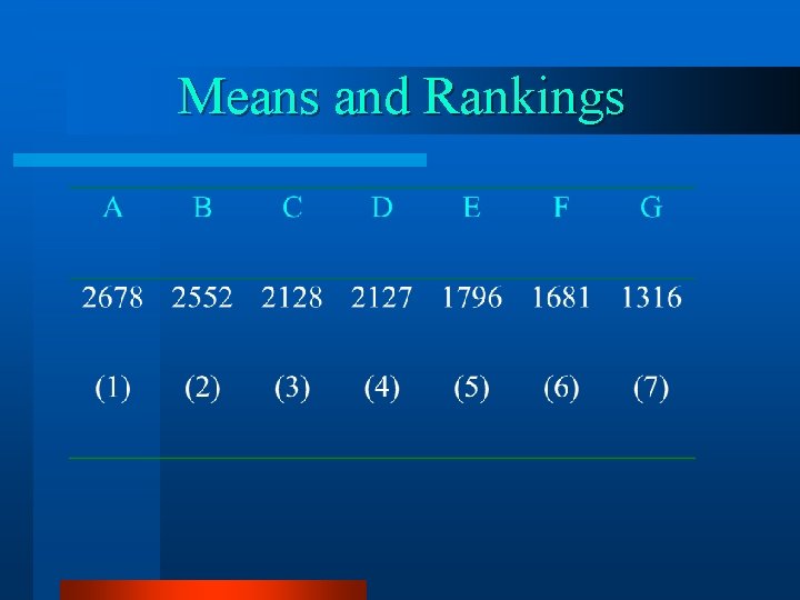
Means and Rankings

Multiple t-Test sed[x] = (2 2/n) (2 x 94, 773/4) |XA - XB|/sed[x] >= tp/2

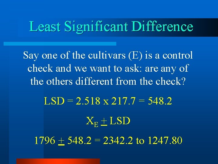
Least Significant Difference |XA - XB|/sed[x] >= tp/2 LSD = tp/2 x sed[x] t 0. 025 = 2. 518 LSD = 2. 518 x 217. 7 = 548. 2

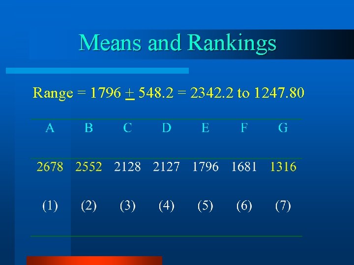
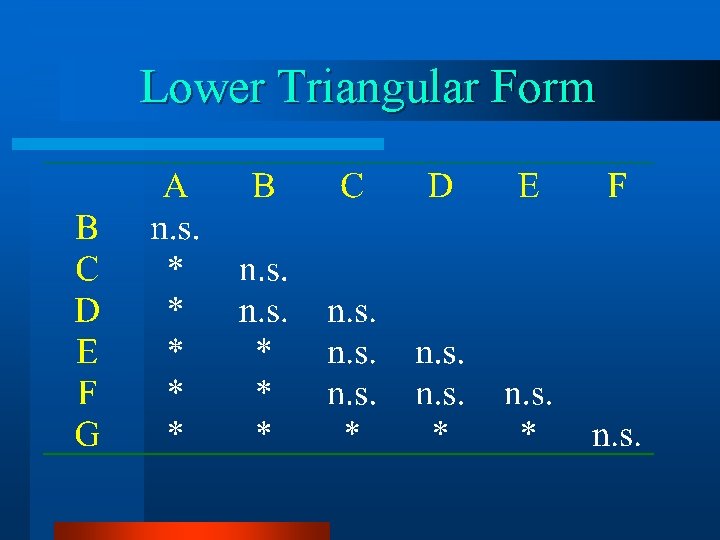
Least Significant Difference Say one of the cultivars (E) is a control check and we want to ask: are any of the others different from the check? LSD = 2. 518 x 217. 7 = 548. 2 XE + LSD 1796 + 548. 2 = 2342. 2 to 1247. 80

Means and Rankings Range = 1796 + 548. 2 = 2342. 2 to 1247. 80

Multiple LSD Comparisons

Lower Triangular Form

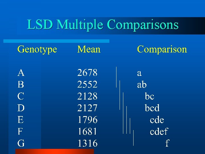
LSD Multiple Comparisons

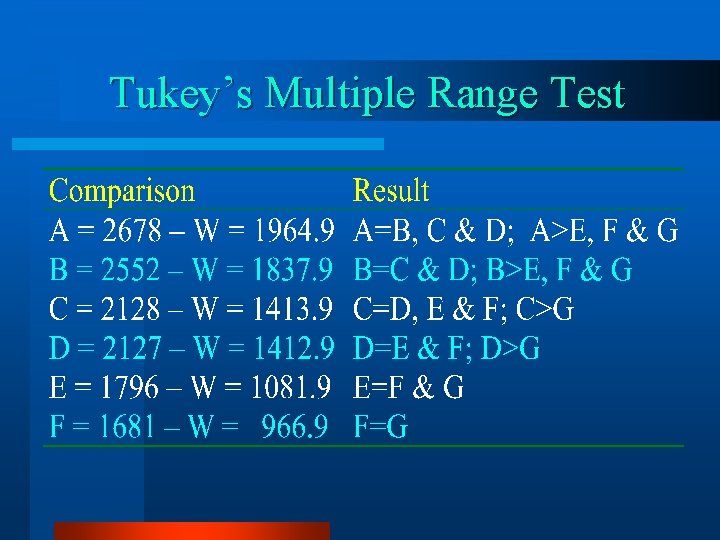
Tukey’s Multiple Range Test W = q(p, f) x se[x] = ( 2/n) (94, 773/4) = 153. 9 W = 4. 64 x 153. 9 = 714. 1

Tukey’s Multiple Range Test

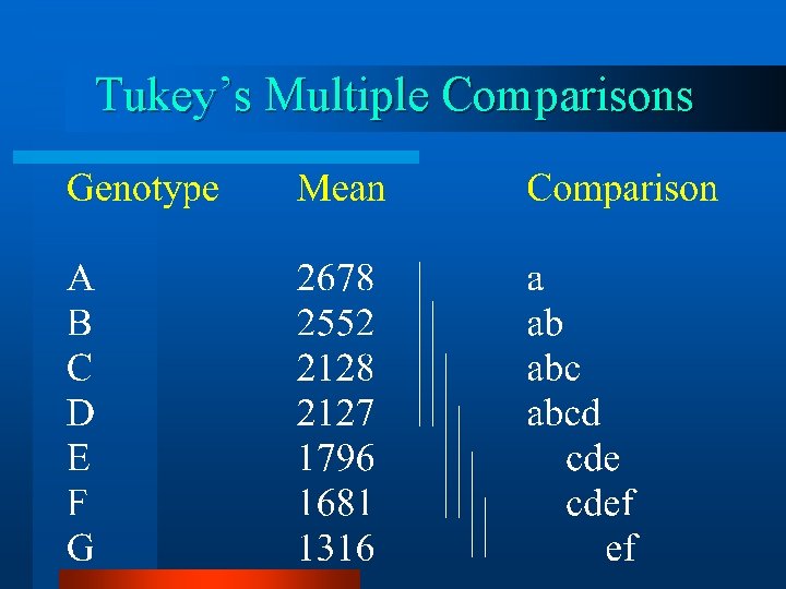
Tukey’s Multiple Comparisons

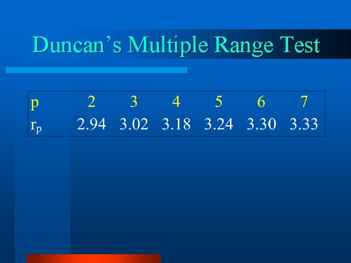
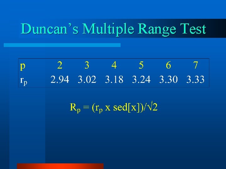
Duncan’s Multiple Range Test

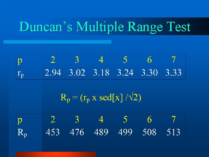
Duncan’s Multiple Range Test

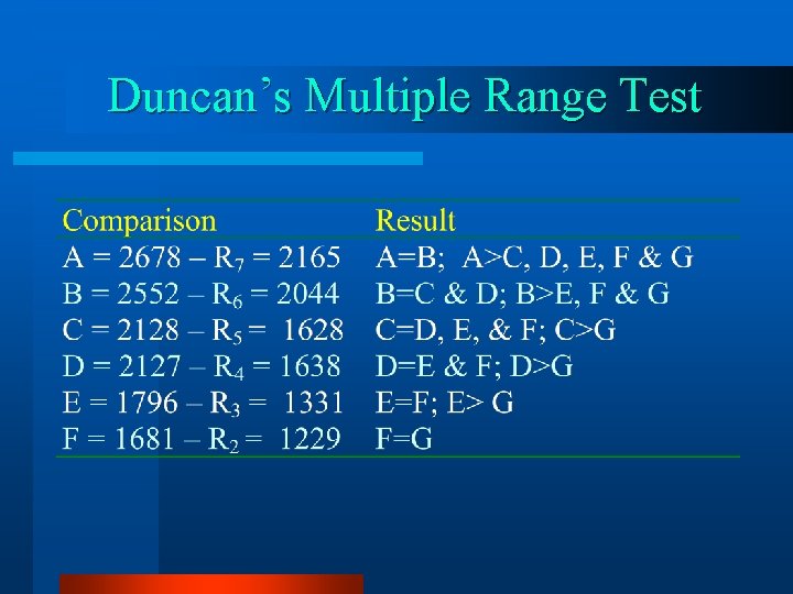
Duncan’s Multiple Range Test

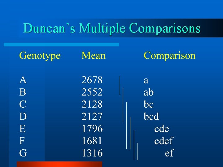
Duncan’s Multiple Range Test

Duncan’s Multiple Comparisons

Orthogonal Contrasts

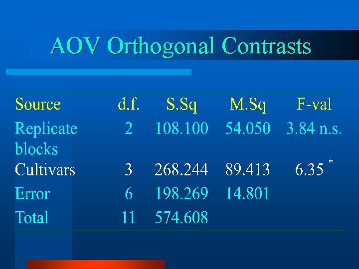
AOV Orthogonal Contrasts

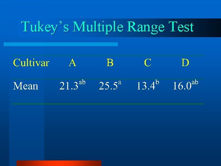
Tukey’s Multiple Range Test

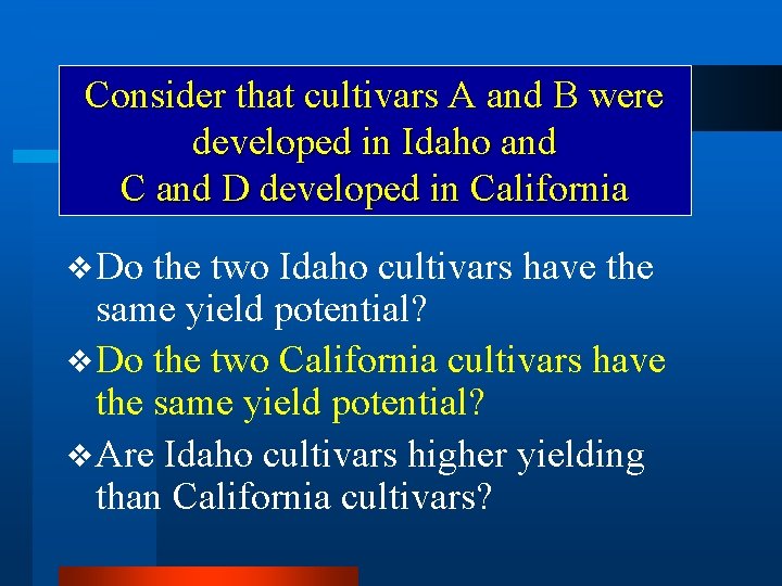
Consider that cultivars A and B were developed in Idaho and C and D developed in California v Do the two Idaho cultivars have the same yield potential? v Do the two California cultivars have the same yield potential? v Are Idaho cultivars higher yielding than California cultivars?

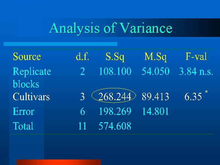
Analysis of Variance

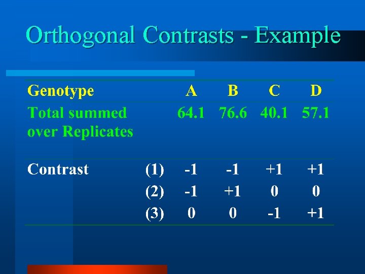
Orthogonality ci = 0 [c 1 i x c 2 i] = 0 -1 -1 +1 +1 -- ci = 0 -1 +1 -- ci = 0 +1 -1 -1 +1 -- ci = 0

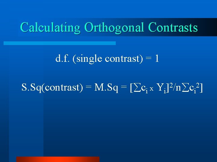
Calculating Orthogonal Contrasts d. f. (single contrast) = 1 S. Sq(contrast) = M. Sq = [ ci x Yi]2/n ci 2]

Orthogonal Contrasts - Example

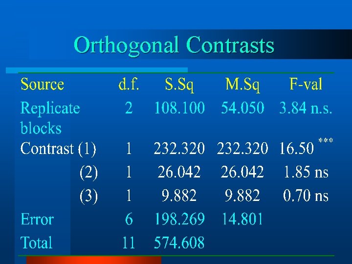
S. Sq = [ ci x Yi]/[n 2 ci ] S. Sq(1) [(-1)64. 1+(-1)76. 6+(1)40. 1+(1)47. 8]2/ n ci 2 = 52. 82/(3 x 4) = 232. 32

S. Sq(2) [(-1)x 64. 1+(+1) x 76. 6]2/(3 x 2) 26. 04 S. Sq(3) [(-1)x 40. 1+(+1) x 47. 8]2/(3 x 2) 9. 88

Orthogonal Contrasts

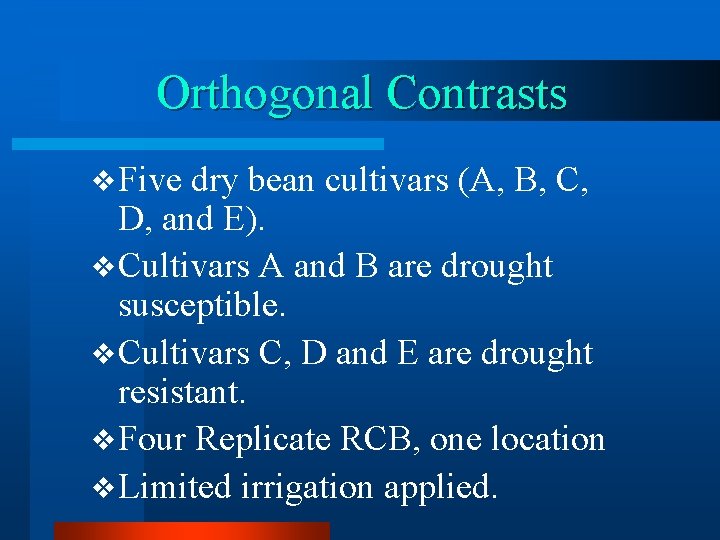
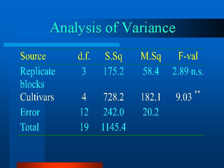
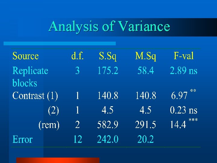
Orthogonal Contrasts v Five dry bean cultivars (A, B, C, D, and E). v Cultivars A and B are drought susceptible. v Cultivars C, D and E are drought resistant. v Four Replicate RCB, one location v Limited irrigation applied.

Analysis of Variance

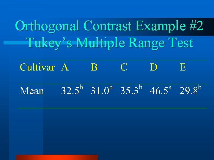
Orthogonal Contrast Example #2 Tukey’s Multiple Range Test

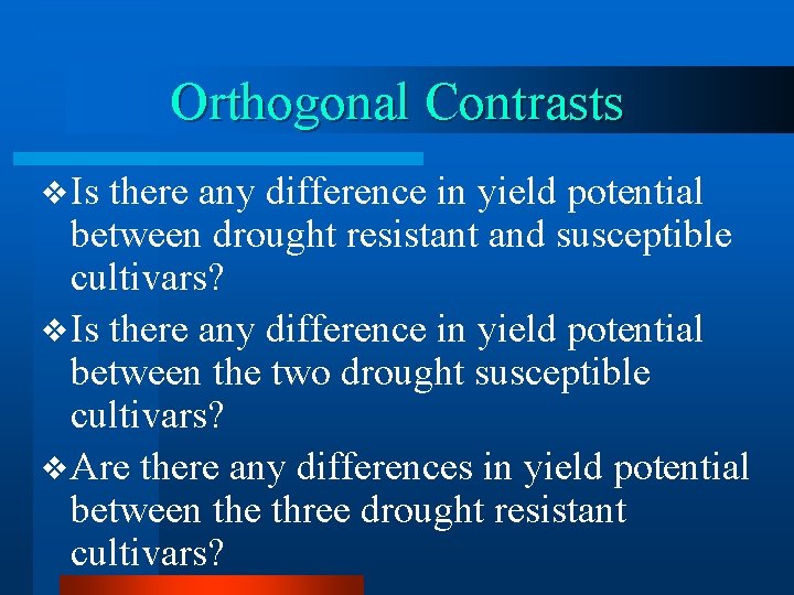
Orthogonal Contrasts v Is there any difference in yield potential between drought resistant and susceptible cultivars? v Is there any difference in yield potential between the two drought susceptible cultivars? v Are there any differences in yield potential between the three drought resistant cultivars?

Orthogonal Contrasts

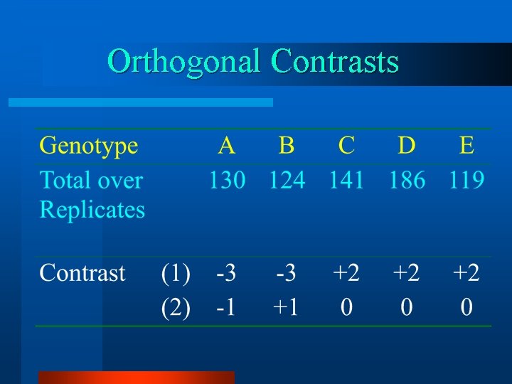
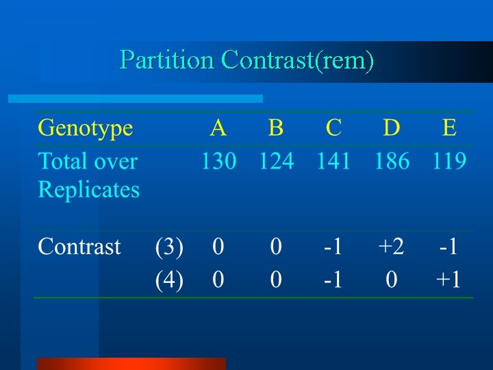
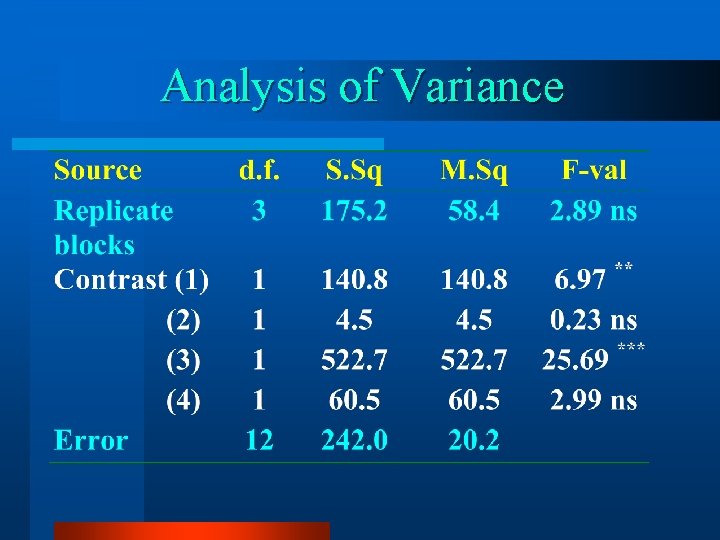
S. Sq(1)= [(-3)130+(-3)124+(2)141+(2)186+(2)119]2 /n ci 2 1302/(4 x 40) = 140. 8 S. Sq(2)= [(-1)130+(+1)124]2 /n ci 2 62/(4 x 2) = 4. 5 S. Sq(Rem) = S. Sq(Cult)-S. Sq(1)-S. Sq(2) 728. 2 -140. 8 -4. 5 = 582. 9 (with 2 d. f. )

Analysis of Variance

Partition Contrast(rem)

Analysis of Variance

Alternative Contrasts !!!!

S. Sq(1)= [(-3)130+(-3)124+(2)141+(2)186+(2)119]2 /n ci 2 1302/(4 x 40) = 140. 8 S. Sq(2)= [(-1)130+(-1)124+(-1)141+(4)186+(-1)119]2 /n ci 2 2302/(4 x 20) = 661. 2 S. Sq(Rem) = S. Sq(Cult)-S. Sq(1)-S. Sq(2) 728. 2 -140. 8 -661. 2 = -73. 8 (Oops !!!) (with 2 d. f. )

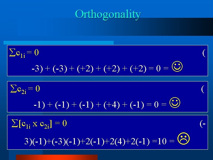
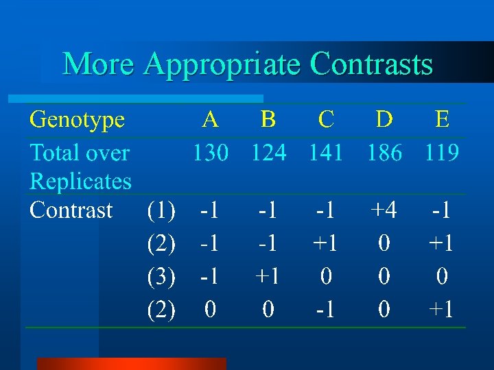
Orthogonality c 1 i = 0 ( c 2 i = 0 ( [c 1 i x c 2 i] = 0 (- -3) + (+2) = 0 = -1) + (-1) + (+4) + (-1) = 0 = 3)(-1)+(-3)(-1)+2(4)+2(-1) =10 =

More Appropriate Contrasts

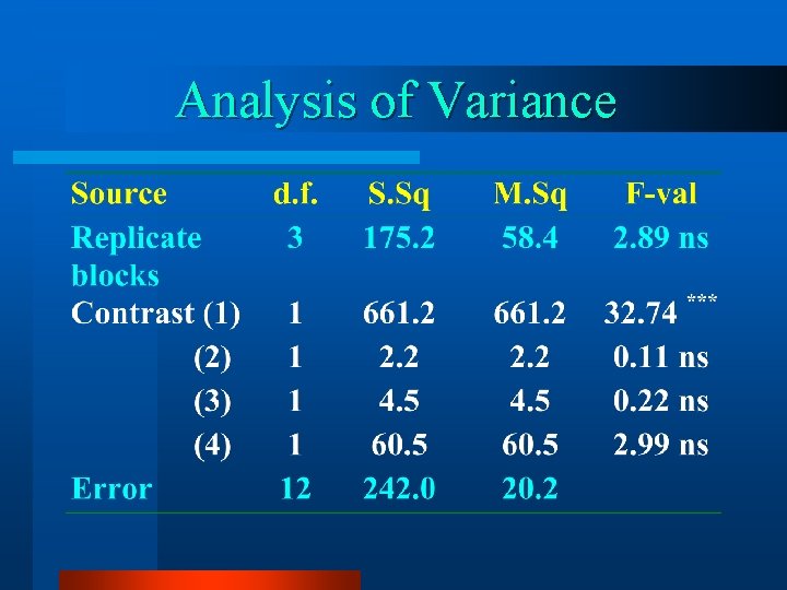
Analysis of Variance

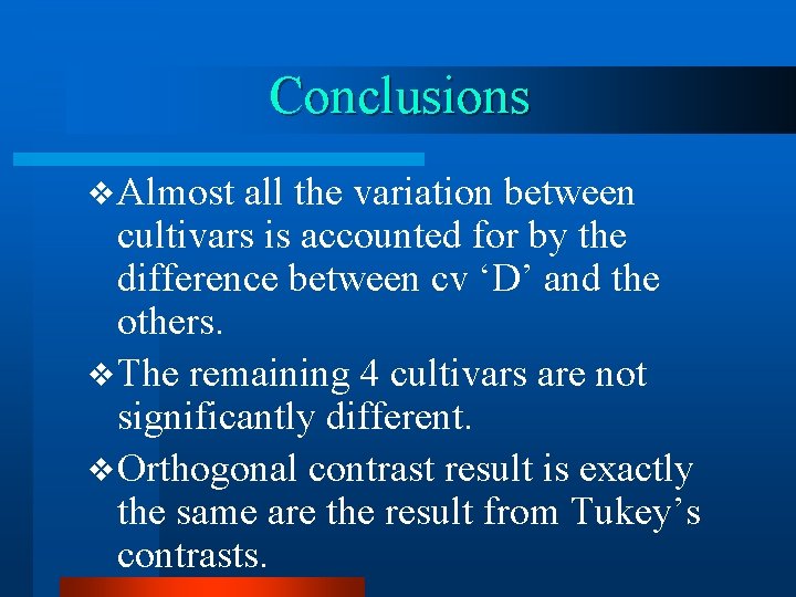
Conclusions v Almost all the variation between cultivars is accounted for by the difference between cv ‘D’ and the others. v The remaining 4 cultivars are not significantly different. v Orthogonal contrast result is exactly the same are the result from Tukey’s contrasts.

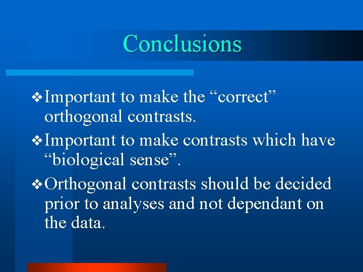
Conclusions v Important to make the “correct” orthogonal contrasts. v Important to make contrasts which have “biological sense”. v Orthogonal contrasts should be decided prior to analyses and not dependant on the data.

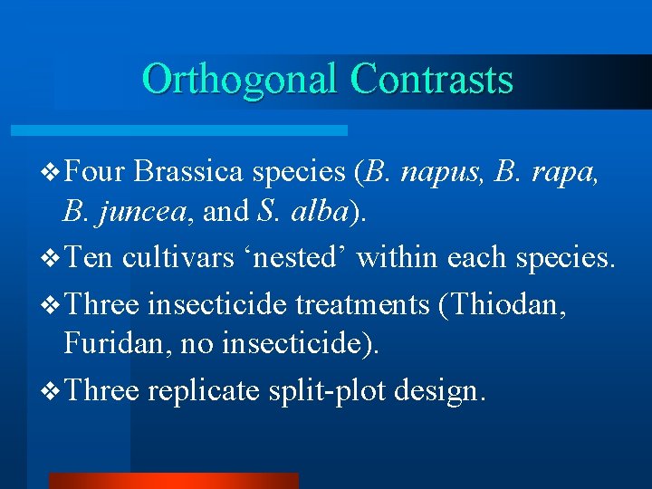
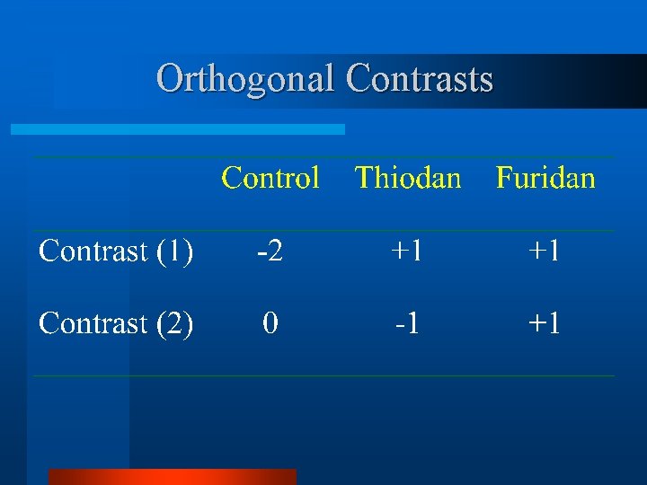
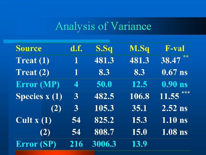
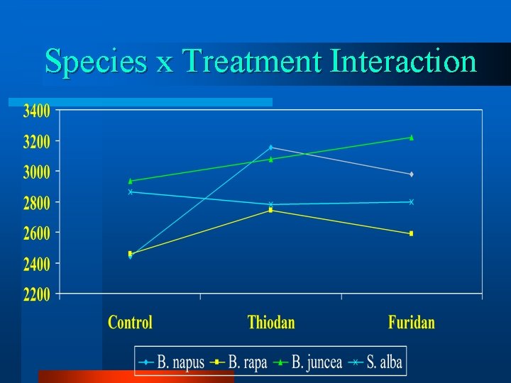
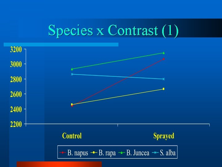
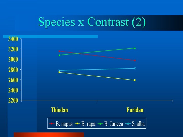
Orthogonal Contrasts v Four Brassica species (B. napus, B. rapa, B. juncea, and S. alba). v Ten cultivars ‘nested’ within each species. v Three insecticide treatments (Thiodan, Furidan, no insecticide). v Three replicate split-plot design.

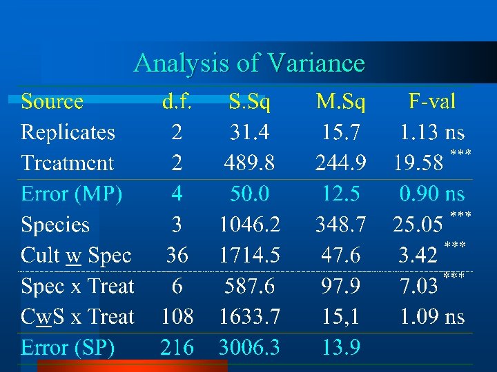
Analysis of Variance

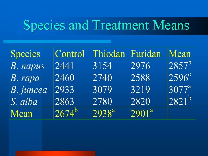
Species and Treatment Means

Orthogonal Contrasts

Orthogonal Contrasts

Analysis of Variance

Species x Treatment Interaction

Species x Contrast (1)

Species x Contrast (2)

More Orthogonal Contrasts … Trend Analyses

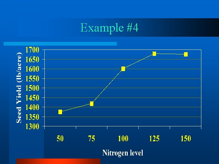
Aim of Analyses of Variance v Detect significant differences between treatment means. v Determine trends that may exist as a result of varying specific factor levels.

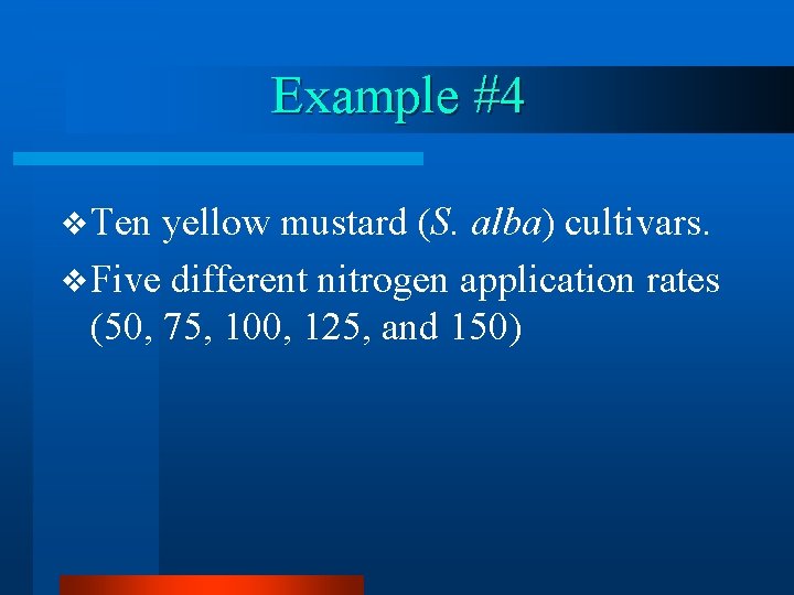
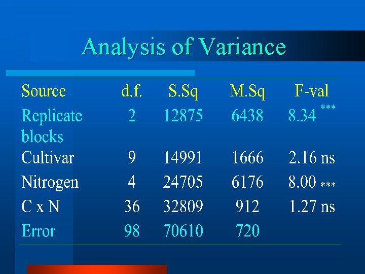
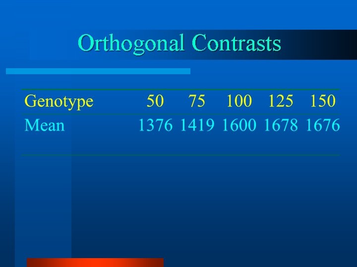
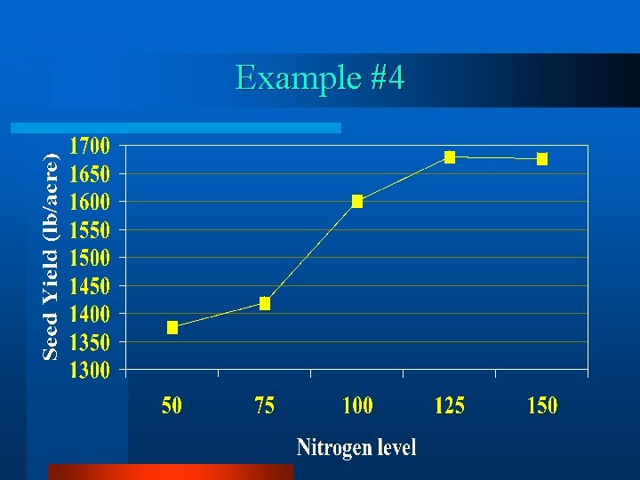
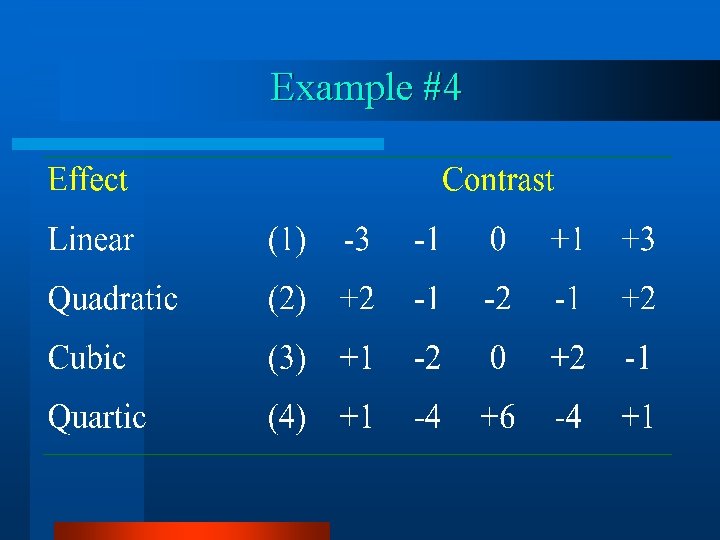
Example #4 v Ten yellow mustard (S. alba) cultivars. v Five different nitrogen application rates (50, 75, 100, 125, and 150)

Analysis of Variance

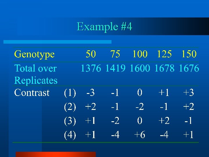
Orthogonal Contrasts

Example #4

Example #4

Example #4

Analysis of Variance

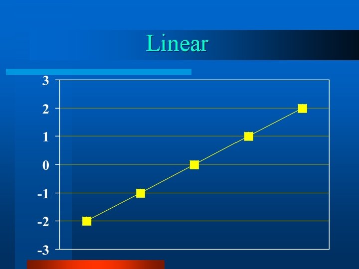
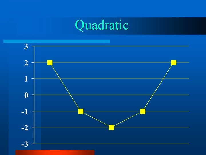
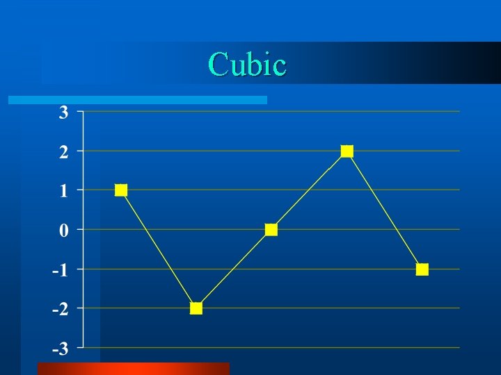
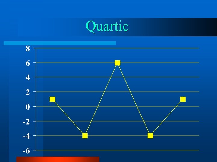
Trend Analyses v. The F-value associates with a trend contrast is significant. v. All higher order trend contrasts are not significant.

Example #4

Linear

Quadratic

Cubic

Quartic

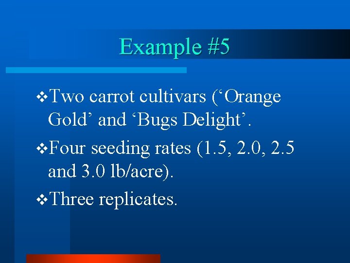
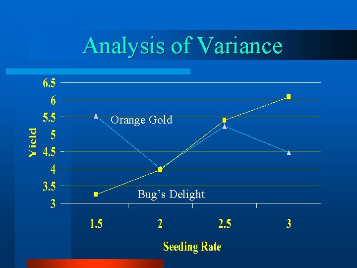
Example #5 v. Two carrot cultivars (‘Orange Gold’ and ‘Bugs Delight’. v. Four seeding rates (1. 5, 2. 0, 2. 5 and 3. 0 lb/acre). v. Three replicates.

Example #5

Analysis of Variance

Analysis of Variance

Analysis of Variance Orange Gold Bug’s Delight

End of Analyses of Variance Section