FiveMinute Check over Lesson 2 1 ThenNow New

Five-Minute Check (over Lesson 2 -1) Then/Now New Vocabulary Example 1: Graph Transformations of Monomial Functions Key Concept: Leading Term Test for Polynomial End Behavior Example 2: Apply the Leading Term Test Key Concept: Zeros and Turning Points of Polynomial Functions Example 3: Zeros of a Polynomial Function Key Concept: Quadratic Form Example 4: Zeros of a Polynomial Function in Quadratic Form Example 5: Polynomial Function with Repeated Zeros Key Concept: Repeated Zeros of Polynomial Functions Example 6: Graph a Polynomial Function Example 7: Real-World Example: Model Data Using Polynomial Functions

Over Lesson 2 -1 A. Graph f (x) = 3 x 3. A. C. B. D.

Over Lesson 2 -1 B. Analyze f (x) = 3 x 3. A. D = (–∞, ∞) R = [0, ∞), intercept: 0, , continuous for all real numbers, decreasing: (–∞, 0) , increasing: (0, ∞) B. D = (–∞, ∞) R = (–∞, ∞), intercept: 0, , continuous for all real numbers, decreasing: (–∞, 0), increasing: (0, ∞) C. D = (–∞, ∞) R = (–∞, ∞), intercept: 0, , continuous for all real numbers, decreasing: (–∞, ∞) D. D = (–∞, ∞) R = (–∞, ∞), intercept: 0, continuous for all real numbers, increasing: (–∞, ∞) ,

Over Lesson 2 -1 Solve A. 7 B. 3, 7 C. D. no solution .

Over Lesson 2 -1 Solve A. – 14 B. – 2 C. 88 D. no solution .

Over Lesson 2 -1 A. – 3, 4 B. 3 C. 6, 1 D. 6

You analyzed graphs of functions. (Lesson 1 -2) • Graph polynomial functions. • Model real-world data with polynomial functions.

• polynomial function • quadratic form • polynomial function of degree n • repeated zero • leading coefficient • leading-term test • quartic function • turning point • multiplicity

Graph Transformations of Monomial Functions A. Graph f (x) = (x – 3)5. This is an odd-degree function, so its graph is similar to the graph of y = x 3. The graph of f(x) = (x – 3)5 is the graph of y = x 5 translated 3 units to the right. Answer:

Graph Transformations of Monomial Functions B. Graph f (x) = x 6 – 1. This is an even-degree function, so its graph is similar to the graph of y = x 2. The graph of f(x) = x 6 – 1 is the graph of y = x 6 translated 1 unit down. Answer:

Graph f (x) = 2 + x 3. A. C. B. D.

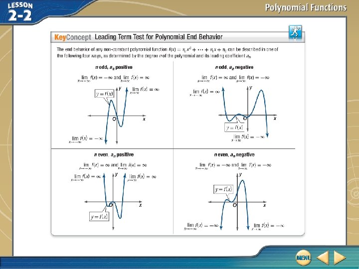
Apply the Leading Term Test A. Describe the end behavior of the graph of f (x) = 3 x 4 – x 3 + x 2 + x – 1 using limits. Explain your reasoning using the leading term test. The degree is 4, and the leading coefficient is 3. Because the degree is even and the leading coefficient is positive, . Answer:

Apply the Leading Term Test B. Describe the end behavior of the graph of f (x) = – 3 x 2 + 2 x 5 – x 3 using limits. Explain your reasoning using the leading term test. Write in standard form as f (x) = 2 x 5 – x 3 – 3 x 2. The degree is 5, and the leading coefficient is 2. Because the degree is odd and the leading coefficient is positive, . Answer:

Apply the Leading Term Test C. Describe the end behavior of the graph of f (x) = – 2 x 5 – 1 using limits. Explain your reasoning using the leading term test. The degree is 5 and the leading coefficient is – 2. Because the degree is odd and the leading coefficient is negative, . Answer:

Describe the end behavior of the graph of g (x) = – 3 x 5 + 6 x 3 – 2 using limits. Explain your reasoning using the leading term test. A. Because the degree is odd and the leading coefficient negative, . B. Because the degree is odd and the leading coefficient negative, . C. Because the degree is odd and the leading coefficient negative, . D. Because the degree is odd and the leading coefficient negative, .

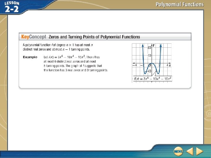
Zeros of a Polynomial Function State the number of possible real zeros and turning points of f (x) = x 3 + 5 x 2 + 4 x. Then determine all of the real zeros by factoring. The degree of the function is 3, so f has at most 3 distinct real zeros and at most 3 – 1 or 2 turning points. To find the real zeros, solve the related equation f (x) = 0 by factoring. x 3 + 5 x 2 + 4 x = 0 Set f (x) equal to 0. x(x 2 + 5 x + 4) = 0 Factor the greatest common factor, x. x(x + 4)(x + 1) = 0 Factor completely.

Zeros of a Polynomial Function So, f has three distinct real zeros, x = 0, x = – 4, and x = – 1. This is consistent with a cubic function having at most 3 distinct real zeros. CHECK You can use a graphing calculator to graph f (x) = x 3 + 5 x 2 + 4 x and confirm these zeros. Additionally, you can see that the graph has 2 turning points, which is consistent with cubic functions having at most 2 turning points.

Zeros of a Polynomial Function Answer: The degree is 3, so f has at most 3 distinct real zeros and at most 2 turning points. f (x) = x 3 + 5 x 2 + 4 x = x (x + 1)(x + 4), so f has three zeros, x = 0, x = – 1, and x = – 4.

State the number of possible real zeros and turning points of f (x) = x 4 – 13 x 2 + 36. Then determine all of the real zeros by factoring. A. 4 possible real zeros, 3 turning points; zeros 2, – 2, 3, – 3 B. 4 possible real zeros, 2 turning points; zeros 4, 9 C. 3 possible real zeros, 2 turning points; zeros 2, 3 D. 4 possible real zeros, 4 turning points; zeros – 2, – 3

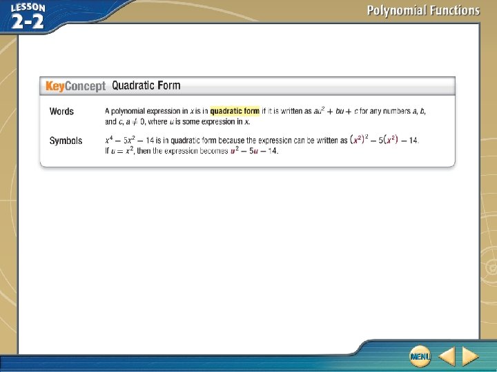
Zeros of a Polynomial Function in Quadratic Form State the number of possible real zeros and turning points for h (x) = x 4 – 4 x 2 + 3. Then determine all of the real zeros by factoring. The degree of the function is 4, so h has at most 4 distinct real zeros and at most 4 – 1 or 3 turning points. This function is in quadratic form because x 4 – 4 x 2 + 3 = (x 2)2 – 4(x 2) + 3. Let u = x 2. (x 2)2 – 4(x 2) + 3 = 0 Set h(x) equal to 0. u 2 – 4 u + 3 = 0 Substitute u for x 2. (u – 3)(u – 1) = 0 Factor the quadratic expression.

Zeros of a Polynomial Function in Quadratic Form (x 2 – 3)(x 2 – 1) = 0 Substitute x 2 for u. Factor completely. Zero Product Property or x + 1 = 0 or x – 1 = 0 , x = – 1, x = 1 Solve for x. h has four distinct real zeros, , – 1, and 1. This is consistent with a quartic function. The graph of h (x) = x 4 – 4 x 2 + 3 confirms this. Notice that there are 3 turning points, which is also consistent with a quartic function.

Zeros of a Polynomial Function in Quadratic Form Answer: The degree is 4, so h has at most 4 distinct real zeros and at most 3 turning points. h (x) = x 4 – 4 x 2 + 3 = (x 2 – 3)(x – 1)(x + 1), so h has four distinct real zeros, x = – 1, and x = 1.

State the number of possible real zeros and turning points of g (x) = x 5 – 5 x 3 – 6 x. Then determine all of the real zeros by factoring. A. 3 possible real zeros, 2 turning points; real zeros 0, – 1, 6 B. 5 possible real zeros, 4 turning points; real zeros 0, C. 3 possible real zeros, 3 turning points; real zeros 0, – 1, . D. 5 possible real zeros, 4 turning points; real zeros 0, 1, – 1,

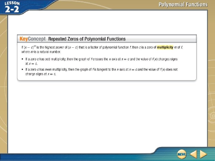
Polynomial Function with Repeated Zeros State the number of possible real zeros and turning points of h (x) = x 4 + 5 x 3 + 6 x 2. Then determine all of the real zeros by factoring. The degree of the function is 4, so it has at most 4 distinct real zeros and at most 4 – 1 or 3 turning points. Find the real zeros. x 4 + 5 x 3 + 6 x 2 = 0 Set h(x) equal to 0. x 2(x 2 + 5 x + 6) = 0 Factor the greatest common factor, x 2(x + 3)(x + 2) = 0 Factor completely.

Polynomial Function with Repeated Zeros The expression above has 4 factors, but solving for x yields only 3 distinct real zeros, x = 0, x = – 3, and x = – 2. Of the zeros, x = 0 is repeated. The graph of h (x) = x 4 + 5 x 3 + 6 x 2 shown here confirms these zeros and shows that h has three turning points. Notice that at x = – 3 and x = – 2, the graph crosses the x-axis, but at x = 0, the graph is tangent to the x-axis.

Polynomial Function with Repeated Zeros Answer: The degree is 4, so h has at most 4 distinct real zeros and at most 3 turning points. h (x) = x 4 + 5 x 3 + 6 x 2 = x 2(x + 2)(x + 3), so h has three zeros, x = 0, x = – 2, and x = – 3. Of the zeros, x = 0 is repeated.

State the number of possible real zeros and turning points of g (x) = x 4 – 4 x 3 + 4 x 2. Then determine all of the real zeros by factoring. A. 4 possible real zeros, 3 turning points; real zeros 0, 2 B. 4 possible real zeros, 3 turning points; real zeros 0, 2, – 2 C. 2 possible real zeros, 1 turning point; real zeros 2, – 2 D. 4 possible real zeros, 3 turning points; real zeros 0, – 2

Graph a Polynomial Function A. For f (x) = x(3 x + 1)(x – 2) 2, apply the leadingterm test. The product x(3 x + 1)(x – 2)2 has a leading term of x(3 x)(x)2 or 3 x 4, so f has degree 4 and leading coefficient 3. Because the degree is even and the leading coefficient is positive, . Answer:

Graph a Polynomial Function B. For f (x) = x(3 x + 1)(x – 2) 2, determine the zeros and state the multiplicity of any repeated zeros. The distinct real zeros are x = 0, x = The zero at x = 2 has multiplicity 2. Answer: 0, , 2 (multiplicity: 2) , and x = 2.

Graph a Polynomial Function C. For f (x) = x(3 x + 1)(x – 2) 2, find a few additional points. Choose x-values that fall in the intervals determined by the zeros of the function. Answer: (– 1, 18), (– 0. 1, – 0. 3087), (1, 4), (3, 30)

Graph a Polynomial Function D. For f (x) = x(3 x + 1)(x – 2) 2, graph the function. Plot the points you found. The end behavior of the function tells you that the graph eventually rises to the left and to the right. You also know that the graph crosses the x-axis at nonrepeated zeros x = and x = 0, but does not cross the x-axis at repeated zero x = 2, because its multiplicity is even. Draw a continuous curve through the points as shown in the figure.

Graph a Polynomial Function Answer:

Determine the zeros and state the multiplicity of any repeated zeros for f (x) = 3 x(x + 2)2(2 x – 1)3. A. 0, – 2 (multiplicity 2), B. 2 (multiplicity 2), – C. 4 (multiplicity 2), D. – 2 (multiplicity 2), (multiplicity 3)

Model Data Using Polynomial Functions A. POPULATION The table to the right shows a town’s population over an 8 -year period. Year 1 refers to the year 2001, year 2 refers to the year 2002, and so on. Create a scatter plot of the data, and determine the type of polynomial function that could be used to represent the data.

Model Data Using Polynomial Functions Enter the data using the list feature of a graphing calculator. Let L 1 be the number of the year. Then create a scatter plot of the data. The curve of the scatter plot resembles the graph of a cubic equation, so we will use a cubic regression. Answer: cubic function;

Model Data Using Polynomial Functions B. POPULATION The table below shows a town’s population over an 8 -year period. Year 1 refers to the year 2001, year 2 refers to the year 2002, and so on. Write a polynomial function to model the data set. Round each coefficient to the nearest thousandth, and state the correlation coefficient.

Model Data Using Polynomial Functions Using the Cubic. Reg tool on a graphing calculator and rounding each coefficient to the nearest thousandth yields f (x) = 10. 020 x 3 – 176. 320 x 2 + 807. 469 x + 4454. 786. The value of r 2 for the data is 0. 89, which is close to 1, so the model is a good fit. We can graph the complete (unrounded) regression by sending it to the Y= menu. In the Y= menu, pick up this regression equation by entering VARS , Statistics, EQ. Graph this function and the scatter plot in the same viewing window. The function appears to fit the data reasonably well.

Model Data Using Polynomial Functions Answer: f (x) = 10. 020 x 3 – 176. 320 x 2 + 807. 469 x + 4454. 786; r 2 = 0. 89

Model Data Using Polynomial Functions C. POPULATION The table below shows a town’s population over an 8 -year period. Year 1 refers to the year 2001, year 2 refers to the year 2002, and so on. Use the model to estimate the population of the town in the year 2012.

Model Data Using Polynomial Functions Use 12 for the year 2012 and use the CALC feature on a calculator to find f (12). The value of f (12) is 6069. 1926, so the population in 2012 will be about 6069. Answer: 6069

Model Data Using Polynomial Functions D. POPULATION The table below shows a town’s population over an 8 -year period. Year 1 refers to the year 2001, year 2 refers to the year 2002, and so on. Use the model to determine the approximate year in which the population reaches 10, 712.

Model Data Using Polynomial Functions Graph the line y = 10, 712 for Y 2. Then use 5: intersect on the CALC menu to find the point of intersection of y = 10, 712 with f (x). The intersection occurs when x ≈ 15, so the approximate year in which the population will be 10, 712 is 2015. Answer: 2015

BIOLOGY The number of fruit flies that hatched after day x is given in the table. Write a polynomial function to model the data set. Round each coefficient to the nearest thousandth, and state the correlation coefficient. Use the model to estimate the number of fruit flies hatched after 8 days. A. y = 12. 014 x 2 – 72. 940 x + 5. 3; r = 0. 84; 190 B. y = 20. 833 x 3 + 125. 786 x 2 + 251. 238 x + 195. 714; r 2 = 0. 99; 40, 922 C. y = 10 x 4 + 60. 833 x 3 + 141. 5 x 2 + 202. 667 x + 182; r 2 = 1; 82, 966 D. y = 70. 893 x – 20. 672; r = 0. 829; 346

HW 2 -2 + Practice 2 -2 # 1 -49 Odd #110 -113