Fisher Linear Discriminant Analysis All material from data

Fisher Linear Discriminant Analysis All material from “data analysis and business analytics with R, ledolter 2013)

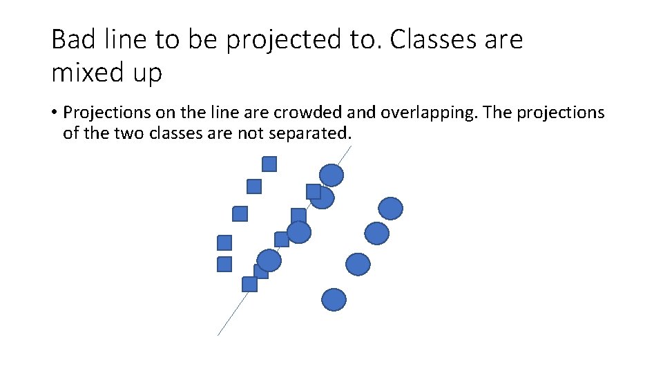
Bad line to be projected to. Classes are mixed up • Projections on the line are crowded and overlapping. The projections of the two classes are not separated.

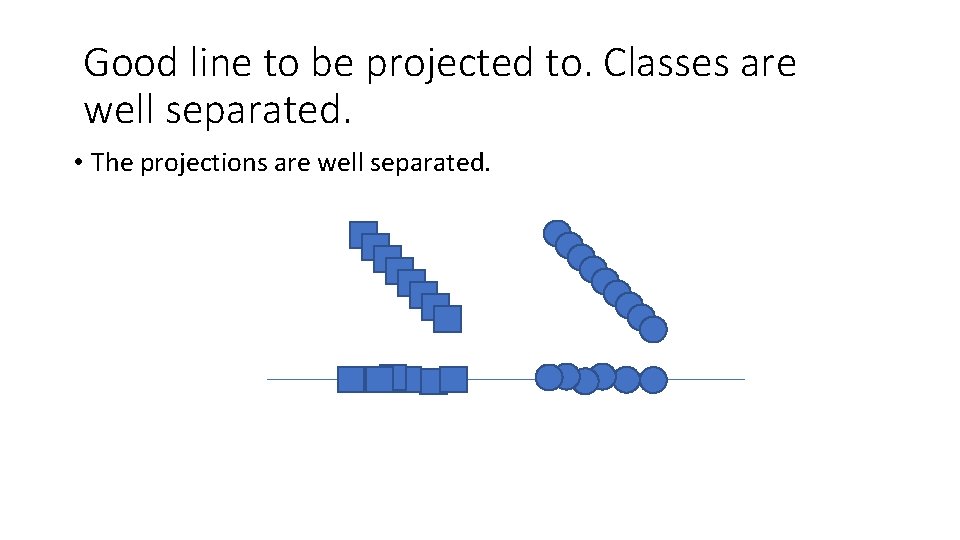
Good line to be projected to. Classes are well separated. • The projections are well separated.

We consider the projection on a line. • Let the line direction be given by a unit vector v. The projection=v^T X V: a unit vector X

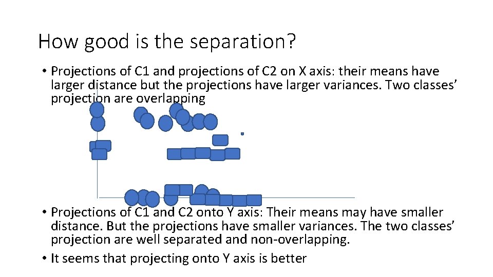
How good is the separation? • Projections of C 1 and projections of C 2 on X axis: their means have larger distance but the projections have larger variances. Two classes’ projection are overlapping • Projections of C 1 and C 2 onto Y axis: Their means may have smaller distance. But the projections have smaller variances. The two classes’ projection are well separated and non-overlapping. • It seems that projecting onto Y axis is better

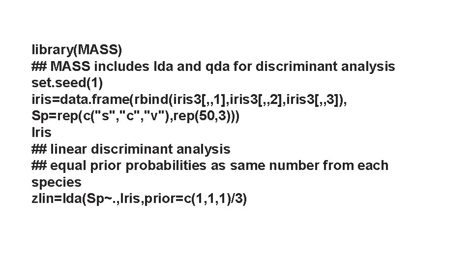
We consider three different species of irises (50 each). Four characteristics are measured on each iris: Sepal. Length, Sepal. Width, Petal. Length, and Petal. Width. The objective is to classify each iris on the basis of these four features.

library(MASS) ## MASS includes lda and qda for discriminant analysis set. seed(1) iris=data. frame(rbind(iris 3[, , 1], iris 3[, , 2], iris 3[, , 3]), Sp=rep(c("s", "c", "v"), rep(50, 3))) Iris ## linear discriminant analysis ## equal prior probabilities as same number from each species zlin=lda(Sp~. , Iris, prior=c(1, 1, 1)/3)

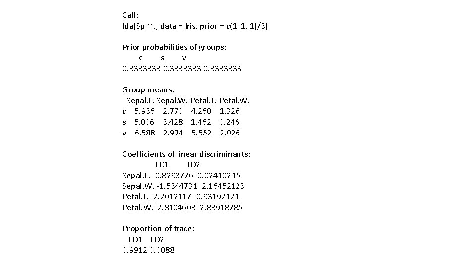
Call: lda(Sp ~. , data = Iris, prior = c(1, 1, 1)/3) Prior probabilities of groups: c s v 0. 3333333 Group means: Sepal. L. Sepal. W. Petal. L. Petal. W. c 5. 936 2. 770 4. 260 1. 326 s 5. 006 3. 428 1. 462 0. 246 v 6. 588 2. 974 5. 552 2. 026 Coefficients of linear discriminants: LD 1 LD 2 Sepal. L. -0. 8293776 0. 02410215 Sepal. W. -1. 5344731 2. 16452123 Petal. L. 2. 2012117 -0. 93192121 Petal. W. 2. 8104603 2. 83918785 Proportion of trace: LD 1 LD 2 0. 9912 0. 0088

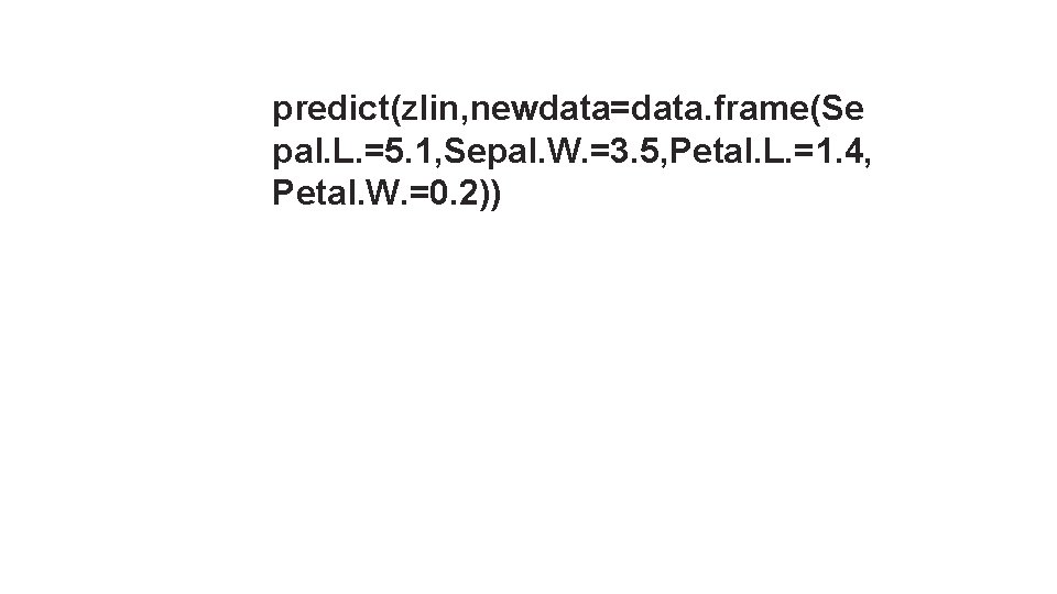
predict(zlin, newdata=data. frame(Se pal. L. =5. 1, Sepal. W. =3. 5, Petal. L. =1. 4, Petal. W. =0. 2))

$`class` [1] s Levels: c s v $posterior cs v 1 3. 896358 e-22 1 2. 611168 e-42 $x LD 1 LD 2 1 -8. 0618 0. 3004206

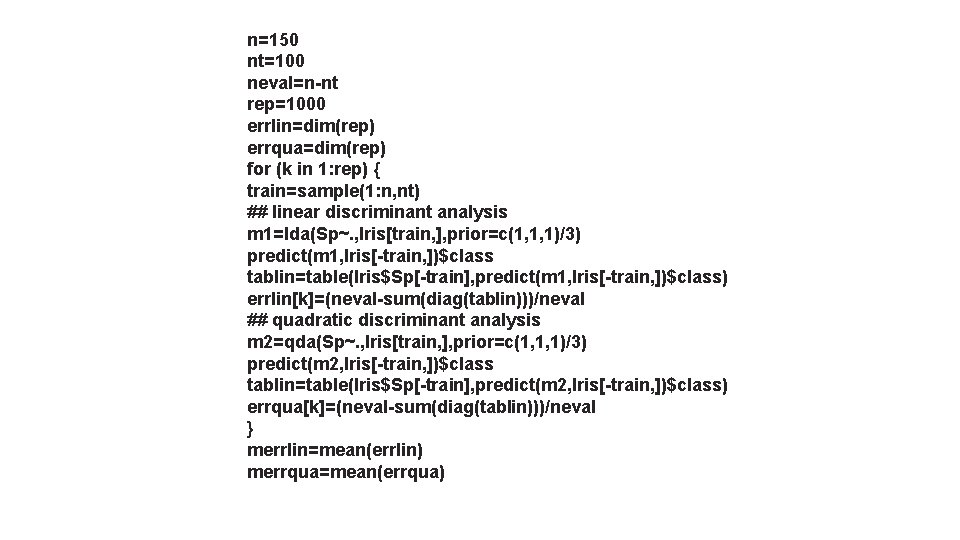
n=150 nt=100 neval=n-nt rep=1000 errlin=dim(rep) errqua=dim(rep) for (k in 1: rep) { train=sample(1: n, nt) ## linear discriminant analysis m 1=lda(Sp~. , Iris[train, ], prior=c(1, 1, 1)/3) predict(m 1, Iris[-train, ])$class tablin=table(Iris$Sp[-train], predict(m 1, Iris[-train, ])$class) errlin[k]=(neval-sum(diag(tablin)))/neval ## quadratic discriminant analysis m 2=qda(Sp~. , Iris[train, ], prior=c(1, 1, 1)/3) predict(m 2, Iris[-train, ])$class tablin=table(Iris$Sp[-train], predict(m 2, Iris[-train, ])$class) errqua[k]=(neval-sum(diag(tablin)))/neval } merrlin=mean(errlin) merrqua=mean(errqua)

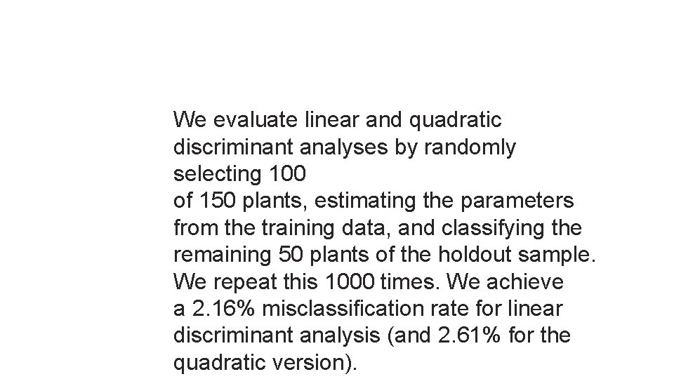
We evaluate linear and quadratic discriminant analyses by randomly selecting 100 of 150 plants, estimating the parameters from the training data, and classifying the remaining 50 plants of the holdout sample. We repeat this 1000 times. We achieve a 2. 16% misclassification rate for linear discriminant analysis (and 2. 61% for the quadratic version).