Fiscal and monetary policy in a closed economy

Fiscal and monetary policy in a closed economy Lecture 5 1

consumption determinants • Current income • Permanent income • Cumulated savings in the past (wealth effect) • Changes in the supply of the consumer credit • expectations 2

Wealth effect • Money and the interest rate have an impact on the wealth • Changes in wealth affect the consumption and the aggregate demand • 2 cases: • 1) increase in wealth caused by changes in real money supply • 2) increase in wealth caused by changes in interest rate. Lower interest rate → higher prices of share and bonds • Why? Market prices of shares and bonds = present value of payments to be received in the future • We have to pay a higher price today to receive any given future payment the lower is the interest rate • the present value ↑if the interest rate↓ 3

The consumption function • The permanent income theory (M. Friedman): consumption proportional to permanent income, not to current income. If household income has fallen temporarily, consumption is not cut so much • Life cycle consumption: consumption is related to income over a longer period than a year, in this case the period of entire lifetime of individual. • Future income affects current consumption. People who expect a higher income will borrow now, people who expect lower income in future (retirement) save to draw savings when they earn little. 4

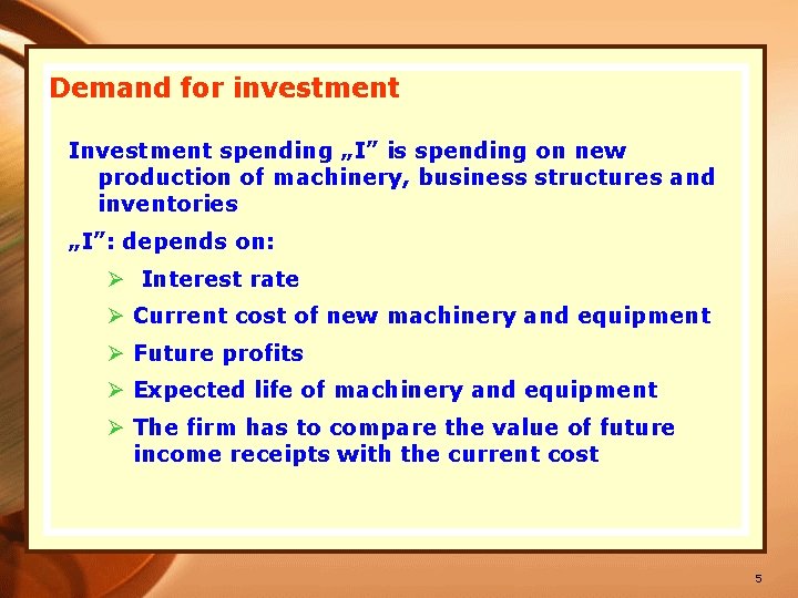
Demand for investment Investment spending „I” is spending on new production of machinery, business structures and inventories „I”: depends on: Ø Interest rate Ø Current cost of new machinery and equipment Ø Future profits Ø Expected life of machinery and equipment Ø The firm has to compare the value of future income receipts with the current cost 5

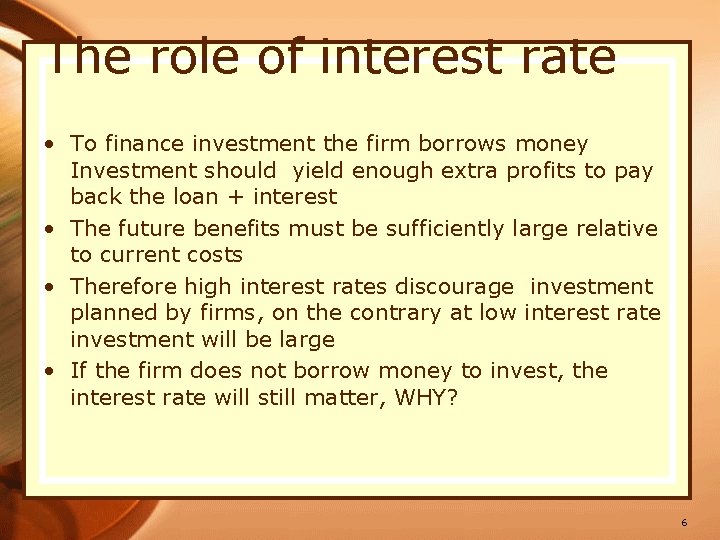
The role of interest rate • To finance investment the firm borrows money Investment should yield enough extra profits to pay back the loan + interest • The future benefits must be sufficiently large relative to current costs • Therefore high interest rates discourage investment planned by firms, on the contrary at low interest rate investment will be large • If the firm does not borrow money to invest, the interest rate will still matter, WHY? 6

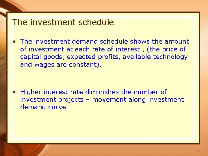
The investment schedule • The investment demand schedule shows the amount of investment at each rate of interest , (the price of capital goods, expected profits, available technology and wages are constant). • Higher interest rate diminishes the number of investment projects – movement along investment demand curve 7

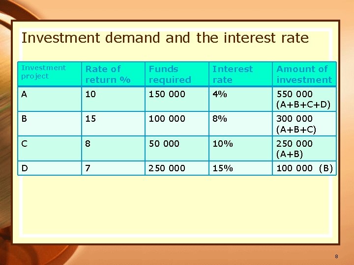
Investment demand the interest rate Investment project Rate of return % Funds required Interest rate Amount of investment A 10 150 000 4% 550 000 (A+B+C+D) B 15 100 000 8% 300 000 (A+B+C) C 8 50 000 10% 250 000 (A+B) D 7 250 000 15% 100 000 (B) 8

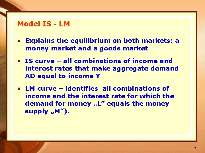
Model IS - LM • Explains the equilibrium on both markets: a money market and a goods market • IS curve – all combinations of income and interest rates that make aggregate demand AD equal to income Y • LM curve – identifies all combinations of income and the interest rate for which the demand for money „L” equals the money supply „M”). 9

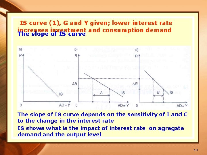
IS curve (1), G and Y given; lower interest rate increases investment and consumption demand The slope of IS curve depends on the sensitivity of I and C to the change in the interest rate IS shows what is the impact of interest rate on agregate demand the output level 10

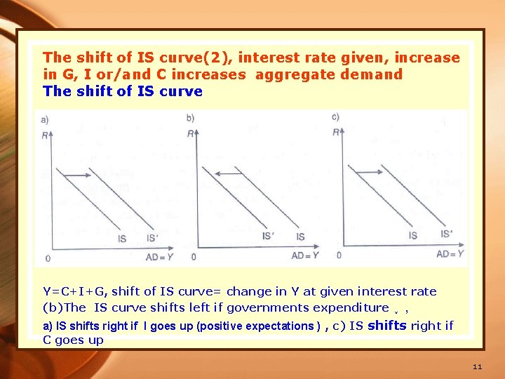
The shift of IS curve(2), interest rate given, increase in G, I or/and C increases aggregate demand The shift of IS curve Y=C+I+G, shift of IS curve= change in Y at given interest rate (b)The IS curve shifts left if governments expenditure ↓ , a) IS shifts right if I goes up (positive expectations ) , c) IS shifts right if C goes up 11

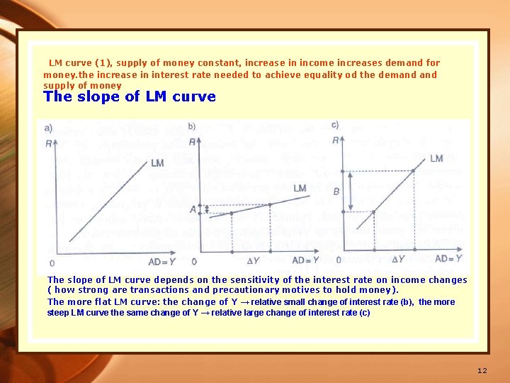
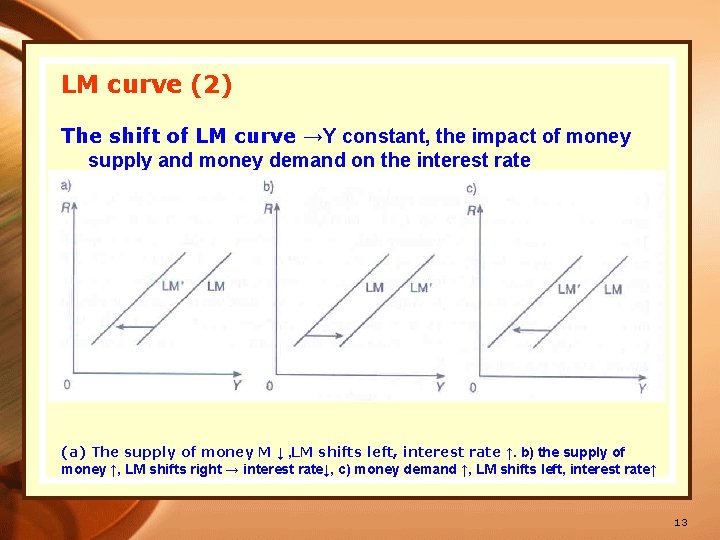
LM curve (1), supply of money constant, increase in income increases demand for money. the increase in interest rate needed to achieve equality od the demand supply of money The slope of LM curve depends on the sensitivity of the interest rate on income changes ( how strong are transactions and precautionary motives to hold money). The more flat LM curve: the change of Y → relative small change of interest rate (b), the more steep LM curve the same change of Y → relative large change of interest rate (c) 12

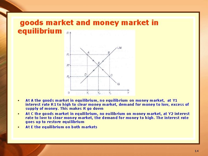
LM curve (2) The shift of LM curve →Y constant, the impact of money supply and money demand on the interest rate (a) The supply of money M ↓ , LM shifts left, interest rate ↑. b) the supply of money ↑, LM shifts right → interest rate↓, c) money demand ↑, LM shifts left, interest rate↑ 13

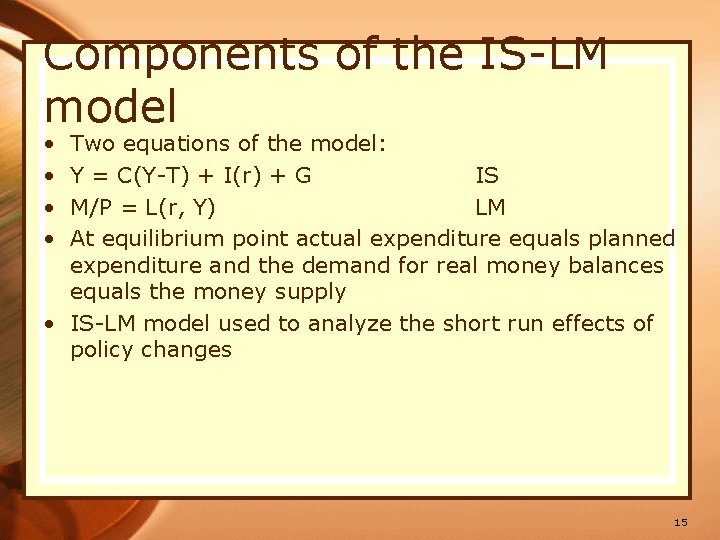
goods market and money market in equilibrium • • • At A the goods market in equilibrium, no equilibrium on money market, at Y 1 interest rate R 1 to high to clear money market, demand for money to low, excess of supply of money. This makes R go down At C the goods market in equilibrium, no euilibrium on money market, at Y 2 interest rate to low to clear money market, the demand for money to high. The interest rate goes up to restore equilibrium At E the equilibrium on both markets 14

Components of the IS-LM model • • Two equations of the model: Y = C(Y-T) + I(r) + G IS M/P = L(r, Y) LM At equilibrium point actual expenditure equals planned expenditure and the demand for real money balances equals the money supply • IS-LM model used to analyze the short run effects of policy changes 15

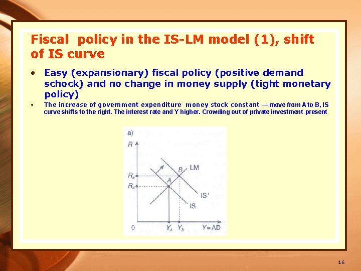
Fiscal policy in the IS-LM model (1), shift of IS curve • Easy (expansionary) fiscal policy (positive demand schock) and no change in money supply (tight monetary policy) • The increase of government expenditure money stock constant → move from A to B, IS curve shifts to the right. The interest rate and Y higher. Crowding out of private investment present 16

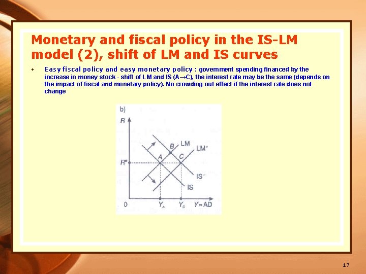
Monetary and fiscal policy in the IS-LM model (2), shift of LM and IS curves • Easy fiscal policy and easy monetary policy : government spending financed by the increase in money stock - shift of LM and IS (A→C), the interest rate may be the same (depends on the impact of fiscal and monetary policy). No crowding out effect if the interest rate does not change 17

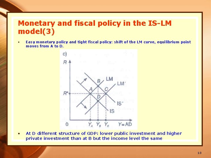
Monetary and fiscal policy in the IS-LM model(3) • Easy monetary policy and tight fiscal policy: shift of the LM curve, equilibrium point moves from A to D. • At D different structure of GDP: lower public investment and higher private investment than at B but the income level the same 18

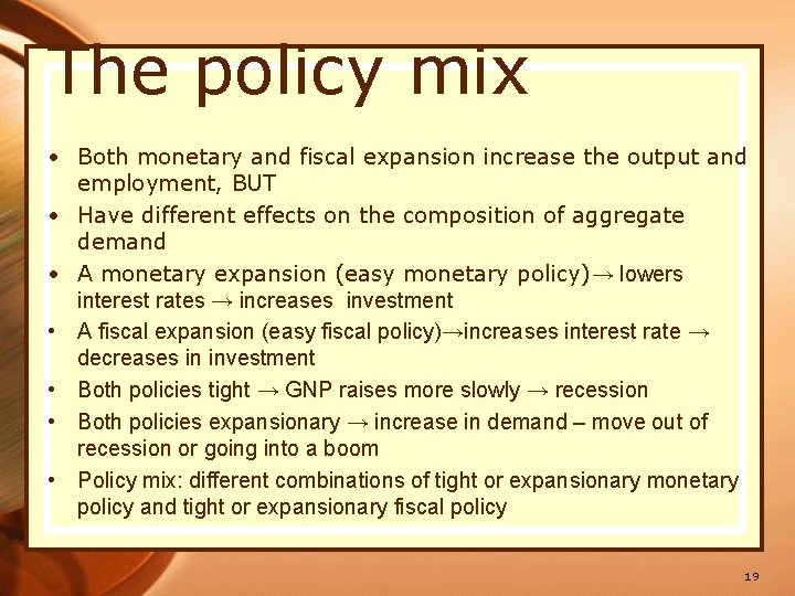
The policy mix • Both monetary and fiscal expansion increase the output and employment, BUT • Have different effects on the composition of aggregate demand • A monetary expansion (easy monetary policy)→ lowers interest rates → increases investment • A fiscal expansion (easy fiscal policy)→increases interest rate → decreases in investment • Both policies tight → GNP raises more slowly → recession • Both policies expansionary → increase in demand – move out of recession or going into a boom • Policy mix: different combinations of tight or expansionary monetary policy and tight or expansionary fiscal policy 19

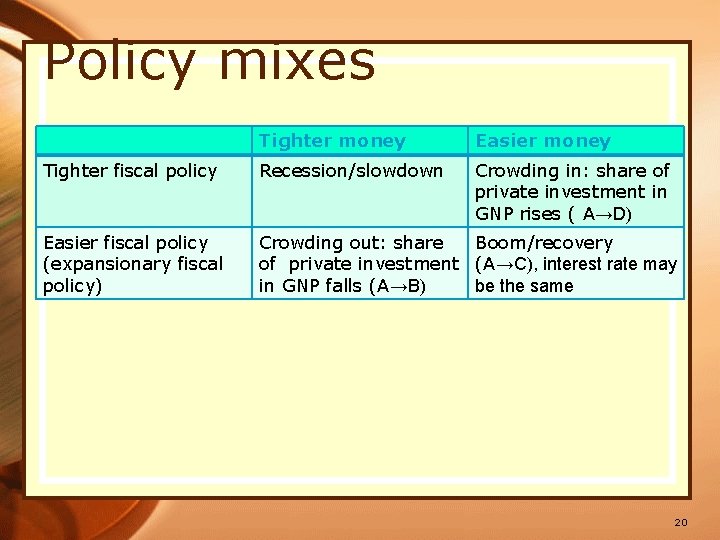
Policy mixes Tighter money Easier money Tighter fiscal policy Recession/slowdown Crowding in: share of private investment in GNP rises ( A→D) Easier fiscal policy (expansionary fiscal policy) Crowding out: share Boom/recovery of private investment (A→C), interest rate may be the same in GNP falls (A→B) 20

Keynesian economics • Analysis of aggregate demand- contribution of J. M. Keynes (1883 -1946) and Keynesians (L. Klein, P. Samuelson, J. Tobin, J. Robinson)Keynesian analysis proceeds on the assumption that the prices level is given and unemployment exists • Critics of Keynesian type economic policy: • Policy works with a lag • Should the monetary and fiscal policy be adjusted continuously? Is fine tuning effective? • The need to include aggregate supply changes 21