First Principles and Machine Learning Calculations of Aqueous


, 289 (2005)")

 Alternatively, run simulation containing both crystal and solvent until")
 A clever new method from the Density of States.")
 Our approach uses no simulations. We compute G*sol under")

")


 • Palmer, D. S. , et al. , Accurate")

 • Combines features of explicit and implicit solvent models.")


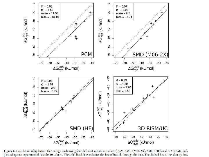


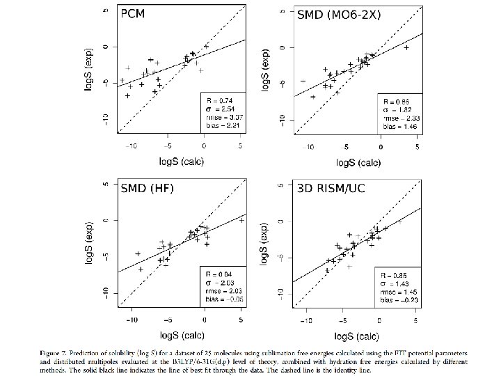


 Image:")


, Neetika Nath, James Mc. Donagh")
- Slides: 64
First Principles and Machine Learning Calculations of Aqueous Solubility Dr John Mitchell University of St Andrews
How should we approach the prediction/estimation/calculation of the aqueous solubility of druglike molecules? Two (apparently) fundamentally different approaches: theoretical chemistry & informatics.
The Two Faces of Computational Chemistry Informatics Theoretical Chemistry
The Two Faces of Computational Chemistry Machine Learning First Principles
First Principles “The problem is difficult, but by making suitable approximations we can solve it at reasonable cost based on our understanding of physics and chemistry”
First Principles “The problem is difficult, but by making suitable approximations we can solve it at reasonable cost based on our understanding of physics and chemistry” Martin Karplus
First Principles “The problem is difficult, but by making suitable approximations we can solve it at reasonable cost based on our understanding of physics and chemistry” Ludwig Boltzmann (1844 -1906)
First Principles • Calculations and simulations based on real physics. • Calculations are either quantum mechanical or use parameters derived from quantum mechanics. • Attempt to model or simulate reality. • Usually Low Throughput.
First Principles • In the context of computing solubility, “first principles” still involves some significant level of approximation.
Drug Disc. Today, 10 (4), 289 (2005)
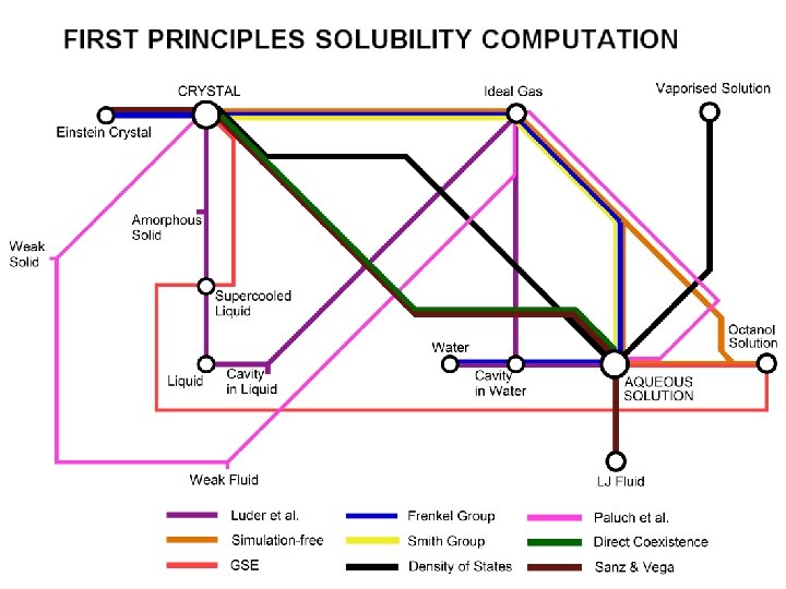
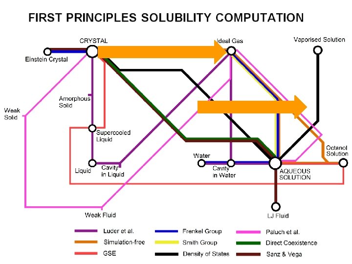
First Principles Solubility Computation
First Principles Solubility Computation (2) Alternatively, run simulation containing both crystal and solvent until equilibrium is reached. “Direct co-existence” “Brute force”
First Principles Solubility Computation (3) A clever new method from the Density of States. Method uses Monte-Carlo Simulations.
First Principles Solubility Computation (4) Our approach uses no simulations. We compute G*sol under some standard conditions, and use this to find the equilibrium constant describing solubility.
Thermodynamic Cycle
OUR DATASET (25 molecules)
We have experimental log. S for all 25 molecules, but can only subdivide into ΔGsub and ΔGhyd for 10 of them.
Thermodynamic Cycle Gas Solution Crystal
Different kinds of theoretical method are used for each part G*sub from lattice energy & a phonon entropy term; DMACRYS using B 3 LYP/6 -31 G(d, p) multipoles and FIT repulsion-dispersion potential. G*hyd
Thermodynamic Cycle Gas Solution Crystal
Sublimation Free Energy Gas Crystal
Sublimation Free Energy Gas Crystal
Sublimation Free Energy Gas Crystal These assumptions may limit accuracy
Sublimation Free Energy Gas Crystal Calculating ΔG*sub is a standard procedure in crystal structure prediction
Results for ΔG*sub Reasonable prediction of ΔG*sub, but small number of molecules. Lattice energies from DMACRYS with FIT atom-atom model potential and B 3 LYP/6 -31 G(d, p) distributed multipoles.
To see the trends in errors, we need to look at more molecules. ΔG sub experimental v ΔG sub predicted 120. 00 R 2 = 0. 3129 100. 00 ΔG sub Predicted 80. 00 Suggests that the assumption 60. 00 G Experimental Vs Predicted Linear(G Experimental Vs Predicted) may limit accuracy 40. 00 RMSE = 22. 4 k. J/mol (46 molecules) 20. 00 20. 00 40. 00 60. 00 ΔG sub Experimental 80. 00 100. 00 120. 00
Thermodynamic Cycle Gas Solution Crystal
Different kinds of theoretical method are used for each part G*sub from lattice energy & a phonon entropy term; DMACRYS using B 3 LYP/6 -31 G(d, p) multipoles and FIT repulsion-dispersion potential. G*hyd from Reference Interaction Site Model with Universal Correction (3 D-RISM/UC).
Reference Interaction Site Model (RISM) • Palmer, D. S. , et al. , Accurate calculations of the hydration free energies of druglike molecules using the reference interaction site model. The Journal of Chemical Physics, 2010. 133(4): p. 044104 -11.
RISM
Reference Interaction Site Model (RISM) • Combines features of explicit and implicit solvent models. • Solvent density is modelled, but no explicit molecular coordinates or dynamics. ~45 CPU mins per compound
Results for ΔG*hyd Error in G*hyd is smaller than in G*sub.
Other Hydration Energy Approaches An alternative methodology here is just to try the various different continuum solvent models available in Gaussian.
log. S 0 from Thermodynamic Cycle Gas Solution Crystal Add the two terms to get ΔG*sol and hence log. S 0.
Results for log. S 0
Conclusions: Theory • • Must calculate G*sub & G*hyd separately; Expt data sparse and errors may be large; RISM is efficient & fairly accurate for G*hyd; Dataset size and composition make comparisons of methods hard; • Not yet matched accuracy of informatics.
Machine Learning “The problem is too difficult to solve using physics and chemistry, so we will design a black box to link structure and solubility”
Informatics and Machine Learning • In general, informatics methods represent phenomena mathematically, but not in a physics-based way. • Inputs and output model are based on an empirically parameterised equation or more elaborate mathematical model. • Do not attempt to simulate reality. • Usually High Throughput.
What Error is Acceptable? • For typically diverse sets of druglike molecules, a “good” QSPR will have an RMSE ≈ 0. 7 to 1. 0 log. S units. • This corresponds to an error range of 4. 0 to 5. 7 k. J/mol in G*sol. • A RMSE > 1. 4 log. S unit is probably unacceptable.
What Error is Acceptable? • A useless model would have an RMSE close to the SD of the test set log. S values: ~ 1. 4 log. S units; • The best possible model would have an RMSE close to the SD resulting from the experimental error in the underlying data: ~ 0. 5 log. S units?
Random Forest A decision tree is like a flow chart
Random Forest Machine Learning Method
Support Vector Machine
Humankind vs The Machines Boobier, Osborn & Mitchell, J Cheminformatics, 9: 63 (2017) Image: scmp. com
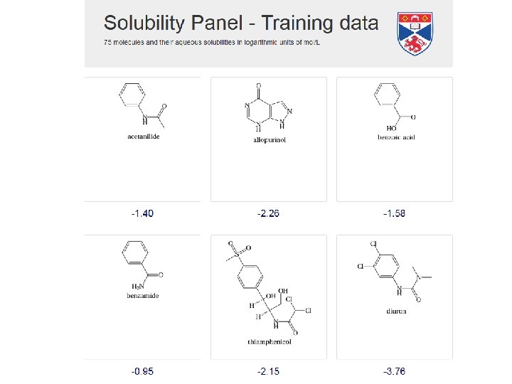
Humankind vs The Machines Challenge is to predict solubilities of 25 molecules given 75 as training data.
Humankind vs The Machines Sent 229 emailed invitations to subject experts and students. Obtained 22 anonymous responses, of those 17 made full sets of predictions.
Humankind vs The Machines 10 machine learning algorithms were given the same training & test sets as the human panel.
0. 99 0. 94 Difference not significant
Machine Learning Algorithms Ranked 1 st 2 nd
Wisdom of Crowds Guess the weight of the cow: Median of individual guesses is a good estimator (after Galton, 1907).
Wisdom of Crowds Guess the solubility of the molecule: Median of all (between 17 & 21) individual human guesses of log. S 0 for a given compound.
1. 09
Wisdom of Crowds Guess the solubility of the molecule: Median of all 10 individual machine guesses of log. S for a given compound.
1. 14 1. 09 Difference not significant
Conclusions: Humans v ML • Best humans and best algorithms perform almost equally; • Consensus of humans and consensus of algorithms perform almost equally; • Both numerically clearly better than first principles on a similar dataset; • Less effective individual human predictors are notably weaker.
Conclusions: Informatics & ML • Expt data: errors unknown (0. 5 -0. 7 log. S 0 units? ) but limit possible accuracy of models; • Cheq. Sol - step in right direction; • Dataset size and composition hinder comparisons of methods; • Numerically better than first principles (but FP not widely validated), at the cost of less insight.
Thanks • SULSA • Tanja van Mourik (St Andrews), Neetika Nath, James Mc. Donagh (now IBM), Rachael Skyner (now Diamond, Oxford), Sam Boobier (now Leeds), Will Kew (now Edinburgh) • Maxim Fedorov, Dave Palmer (Strathclyde) • Laura Hughes (now Stanford), Toni Llinas (AZ), Anne Osbourn (JIC, Norwich)