First Order Representations and Learning coming up later

First Order Representations and Learning coming up later: scalability!

Announcements l PIG assignment (last one) is out l l Added some other examples to the “PIG workflow” lecture, as well as pointers to documentation, etc. PIG has been installed on Gates cluster l l Sample exam questions will be out l l l see docs on cluster on course page soon (Friday? ) think about the non-programming exercises in the HWs also Exam is 4/30 (in-class)

A little history l Tasks you do well: l l l l statistical approaches Recognizing human faces Character recognition (7 vs 4) Simulations of physical events Understanding statements in natural language Proving mathematical theorems Playing chess, Othello, … logical approaches Solving logic puzzles (Soduko)

Logical approaches l “All men are mortal, Socrates is a man, so Socrates is mortal”. l l l quantification: for all, there exists plus logical connectives: and, or, … for all W, X, Y, Z: l l for all X: man(X) mortal(X) man(socrates) father(X, Y) & mother(X, Z) & father(W, Y) & father(W, Z) & W!=X <==> sibling(X, W) for all X: feeds. Young. Milk(X) mammal(X) l for all X: mammal(X) has. Spine(X)

Markov Logic Networks Mostly pilfered from Pedro’s slides

Motivation l l l The real world is complex and uncertain Logic handles complexity Probability handles uncertainty

MLN’s Bold Agenda: “Unify Logical and Statistical AI” Field Logical approach Statistical approach Knowledge representation First-order logic Graphical models Automated reasoning Satisfiability testing Markov chain Monte Carlo (e. g. Gibbs) Machine learning Inductive logic programming Neural networks, …. Planning Markov decision processes Classical planning Natural language Definite clause grammars processing Prob. context-free grammars

Markov Networks: [Review] l Undirected graphical models Smoking Cancer Asthma l Cough Potential functions defined over cliques Smoking Cancer Ф(S, C) False 4. 5 False True 4. 5 True False 2. 7 True 4. 5

Markov Networks l Undirected graphical models Smoking Cancer Asthma l Cough Log-linear model: Weight of Feature i

Inference in Markov Networks l Goal: Compute marginals & conditionals of l l Exact inference is #P-complete Conditioning on Markov blanket is easy: l Gibbs sampling exploits this

MCMC: Gibbs Sampling state ← random truth assignment for i ← 1 to num-samples do for each variable x sample x according to P(x|neighbors(x)) state ← state with new value of x P(F) ← fraction of states in which F is true

Overview l l Motivation Foundational areas l l l l Probabilistic inference [Markov nets] Statistical learning Logical inference Inductive logic programming Putting the pieces together MLNs Applications

Learning Markov Networks l Learning parameters (weights) l l Generatively Discriminatively Learning structure (features) In this tutorial: Assume complete data (If not: EM versions of algorithms)

Generative Weight Learning l l l Maximize likelihood or posterior probability Numerical optimization (gradient or 2 nd order) No local maxima No. of times feature i is true in data Expected no. times feature i is true according to model l Requires inference at each step (slow!)

Pseudo-Likelihood l l l Likelihood of each variable given its neighbors in the data Does not require inference at each step Consistent estimator Widely used in vision, spatial statistics, etc. But PL parameters may not work well for long inference chains

Discriminative Weight Learning l Maximize conditional likelihood of query (y) given evidence (x) No. of true groundings of clause i in data Expected no. true groundings according to model l Approximate expected counts by counts in MAP state of y given x l [Like CRF learning – WC]

Overview l l Motivation Foundational areas l l l l Probabilistic inference [Markov nets] Statistical learning Logical inference Inductive logic programming Putting the pieces together MLNs Applications

First-Order Logic l l l Constants, variables, functions, predicates E. g. : Anna, x, Mother. Of(x), Friends(x, y) Literal: Predicate or its negation Clause: Disjunction of literals Grounding: Replace all variables by constants E. g. : Friends (Anna, Bob) World (model, interpretation): Assignment of truth values to all ground predicates

Inference in First-Order Logic l l “Traditionally” done by theorem proving (e. g. : Prolog) Propositionalization followed by model checking turns out to be faster (often a lot) l l [This was popularized by Kautz & Selman – WC] Propositionalization: Create all ground atoms and clauses Model checking: Satisfiability testing Two main approaches: l l Backtracking (e. g. : DPLL) Stochastic local search (e. g. : Walk. SAT)

Satisfiability l Input: Set of clauses (Convert KB to conjunctive normal form (CNF)) l l l (A v B v ~C)(~B v D) … Output: Truth assignment that satisfies all clauses, or failure The paradigmatic NP-complete problem Solution: Search Key point: Most [random] SAT problems are actually easy Hard region: Narrow range of #Clauses / #Variables

Backtracking l l l Assign truth values by depth-first search Assigning a variable deletes false literals and satisfied clauses Empty set of clauses: Success Empty clause: Failure Additional improvements: l l Unit propagation (unit clause forces truth value) Pure literals (same truth value everywhere)

Stochastic Local Search l l l Uses complete assignments instead of partial Start with random state Flip variables in unsatisfied clauses Hill-climbing: Minimize # unsatisfied clauses Avoid local minima: Random flips Multiple restarts

The Walk. SAT Algorithm for i ← 1 to max-tries do solution = random truth assignment for j ← 1 to max-flips do if all clauses satisfied then return solution c ← random unsatisfied clause with probability p flip a random variable in c else flip variable in c that maximizes number of satisfied clauses return failure

Overview l l Motivation Foundational areas l l l l Probabilistic inference [Markov nets] Statistical learning Logical inference Inductive logic programming Putting the pieces together MLNs Applications

Markov Logic l l Logical language: First-order logic Probabilistic language: Markov networks l l l Learning: l l l Syntax: First-order formulas with weights Semantics: Templates for Markov net features Parameters: Generative or discriminative Structure: ILP with arbitrary clauses and MAP score Inference: l l l MAP: Weighted satisfiability Marginal: MCMC with moves proposed by SAT solver Partial grounding + Lazy inference

Markov Logic: Intuition l l l A logical KB is a set of hard constraints on the set of possible worlds Let’s make them soft constraints: When a world violates a formula, It becomes less probable, not impossible Give each formula a weight (Higher weight Stronger constraint)

Markov Logic: Definition l A Markov Logic Network (MLN) is a set of pairs (F, w) where l l l F is a formula in first-order logic w is a real number Together with a set of constants, it defines a Markov network with l l One node for each grounding of each predicate in the MLN One feature for each grounding of each formula F in the MLN, with the corresponding weight w

Example: Friends & Smokers

Example: Friends & Smokers

Example: Friends & Smokers

Example: Friends & Smokers Two constants: Anna (A) and Bob (B)

Example: Friends & Smokers Two constants: Anna (A) and Bob (B) Smokes(A) Cancer(A) Smokes(B) Cancer(B)

Example: Friends & Smokers Two constants: Anna (A) and Bob (B) Friends(A, A) Smokes(B) Cancer(A) Friends(B, B) Cancer(B) Friends(B, A)

Example: Friends & Smokers Two constants: Anna (A) and Bob (B) Friends(A, A) Smokes(B) Cancer(A) Friends(B, B) Cancer(B) Friends(B, A)

Example: Friends & Smokers Two constants: Anna (A) and Bob (B) Friends(A, A) Smokes(B) Cancer(A) Friends(B, B) Cancer(B) Friends(B, A)

Markov Logic Networks l MLN is template for ground Markov nets l Probability of a world x: Weight of formula i l l l No. of true groundings of formula i in x Typed variables and constants greatly reduce size of ground Markov net Functions, existential quantifiers, etc. Infinite and continuous domains

Relation to Statistical Models l Special cases: l l l Markov networks Markov random fields Bayesian networks Log-linear models Exponential models Max. entropy models Gibbs distributions Boltzmann machines Logistic regression Hidden Markov models Conditional random fields l Obtained by making all predicates zero-arity l Markov logic allows objects to be interdependent (non-i. i. d. )

Relation to First-Order Logic l l l Infinite weights First-order logic Satisfiable KB, positive weights Satisfying assignments = Modes of distribution Markov logic allows contradictions between formulas

<aside> Is this a good thing? l Pros: l l Drawing connections between problems Specifying/visualizing/prototyping new methods … Cons: l l l Robust, general tools are very hard to build for computationally hard tasks This is especially true when learning is involved Eg, MCMC doesn’t work well for large weights

Learning l l Data is a relational database Closed world assumption (if not: EM) Learning parameters (weights) Learning structure (formulas)

Weight Learning l Parameter tying: Groundings of same clause No. of times clause i is true in data Expected no. times clause i is true according to MLN l l Generative learning: Pseudo-likelihood Discriminative learning: Cond. Likelihood l [still just like CRFs - all we need is to do inference efficiently. Here they use a Collins-like method. WC]

Problem 1… Memory Explosion l Problem: If there are n constants and the highest clause arity is c, c the ground network requires O(n ) memory l Solution: Exploit sparseness; ground clauses lazily → Lazy. SAT algorithm [Singla & Domingos, 2006] l [WC: this is a partial solution…. ]

Ground Network Construction network ← Ø queue ← query nodes repeat node ← front(queue) remove node from queue add node to network if node not in evidence then add neighbors(node) to queue until queue = Ø

Example: Friends & Smokers Two constants: Anna (A) and Bob (B) Friends(A, A) Smokes(B) Cancer(A) Friends(B, B) Cancer(B) Friends(B, A)

Problem 2: MAP/MPE Inference l Problem: Find most likely state of world given evidence Query Evidence

MAP/MPE Inference l Problem: Find most likely state of world given evidence

MAP/MPE Inference l Problem: Find most likely state of world given evidence

MAP/MPE Inference l Problem: Find most likely state of world given evidence l This is just the weighted Max. SAT problem Use weighted SAT solver (e. g. , Max. Walk. SAT [Kautz et al. , 1997] ) Potentially faster than logical inference (!) l l

The Max. Walk. SAT Algorithm for i ← 1 to max-tries do solution = random truth assignment for j ← 1 to max-flips do if ∑ weights(sat. clauses) > threshold then return solution c ← random unsatisfied clause with probability p flip a random variable in c else flip variable in c that maximizes ∑ weights(sat. clauses) return failure, best solution found

MCMC is Insufficient for Logic l Problem: Deterministic dependencies break MCMC Near-deterministic ones make it very slow l Solution: Combine MCMC and Walk. SAT → MC-SAT algorithm [Poon & Domingos, 2006]

Current Best Solution: The MCSAT Algorithm l l [Basic idea: figure out how to sample from SAT assignments, and use this as a subroutine for MCMC WC] MC-SAT = MCMC + SAT l l MCMC: Slice sampling with an auxiliary variable for each clause SAT: Wraps around Sample. SAT (a uniform sampler) to sample from highly non-uniform distributions l Sound: Satisfies ergodicity & detailed balance l Efficient: Orders of magnitude faster than Gibbs and other MCMC algorithms

The MC-SAT Algorithm X ( 0 ) A random solution satisfying all hard clauses for k 1 to num_samples M Ø forall Ci satisfied by X ( k – 1 ) With prob. 1 – exp ( – wi ) add Ci to M endfor X ( k ) A uniformly random solution satisfying M endfor

The MC-SAT Algorithm l Sound: Satisfies ergodicity and detailed balance Assuming we have a perfect uniform sampler l Of course, we don’t (since the problem is #P-hard) But there is an approximate uniform sampler [Wei et al. 2004] l l Sample. SAT = Walk. SAT + Simulated annealing Trade off uniformity vs. efficiency by tuning the prob. of WS steps vs. SA steps

Overview l l Motivation Foundational areas l l l l Probabilistic inference [Markov nets] Statistical learning Logical inference Inductive logic programming Putting the pieces together MLNs Applications

Applications l l l l Basics Logistic regression Hypertext classification Information retrieval Entity resolution Hidden Markov models Information extraction l l l l Statistical parsing Semantic processing Bayesian networks Relational models Robot mapping Planning and MDPs Practical tips

Text Classification page = { 1, … , n } word = { … } topic = { … } Topic(page, topic!) Has. Word(page, word) !Topic(p, t) [bias term, since topics are sparse? –WC] Has. Word(p, +w) => Topic(p, +t)

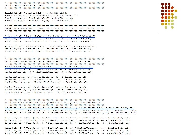
Entity Resolution Problem: Given database, find duplicate records Has. Token(token, field, record) Same. Field(field, record) Same. Record(record, record) TFIDFSim. Greater. Than 0. 8(+t, +f, r’) Has. Token(+t, +f, r) ^ Has. Token(+t, +f, r’) => Same. Field(f, r, r’) => Same. Record(r, r’) ^ Same. Record(r’, r”) => Same. Record(r, r”) TFIDFSim. Greater. Than 0. 6(+t, +f, r’) => Same. Field(f, r, r’) TFIDFSim. Greater. Than 0. 4(+t, +f, r’) => Same. Field(f, r, r’) Etc, etc

Entity Resolution Problem: Given database, find duplicate records Has. Token(token, field, record) Same. Field(field, record) Same. Record(record, record) Has. Token(+t, +f, r) ^ Has. Token(+t, +f, r’) => Same. Field(f, r, r’) => Same. Record(r, r’) ^ Same. Record(r’, r”) => Same. Record(r, r”)

Entity Resolution Can also resolve fields: Has. Token(token, field, record) Same. Field(field, record) Same. Record(record, record) Has. Token(+t, +f, r) ^ Has. Token(+t, +f, r’) => Same. Field(f, r, r’) <=> Same. Record(r, r’) ^ Same. Record(r’, r”) => Same. Record(r, r”) Same. Field(f, r, r’) ^ Same. Field(f, r’, r”) => Same. Field(f, r, r”) P. Singla & P. Domingos, “Entity Resolution with Markov Logic”, in Proc. ICDM-2006.

Hidden Markov Models obs = { Obs 1, … , Obs. N } state = { St 1, … , St. M } time = { 0, … , T } State(state!, time) Obs(obs!, time) State(+s, 0) State(+s, t) => State(+s', t+1) Obs(+o, t) => State(+s, t)

William’s summary l MLNs are a compact, elegant way of describing a Markov network l l Standard learning methods work Network may be very large Inference may be expensive Doesn’t eliminate feature engineering l l E. g. , complicated “feature” predicates Experimental results for joint matching/NER are not that strong overall l Cascading segmentation and then matching improves segmentation, probably not matching But it needs to be carefully restricted (efficiency? ) And it’s no better than a “pseudo” joint model using plausible matches as features