Firewalls and Intrusion Detection Systems David Brumley dbrumleycmu

Firewalls and Intrusion Detection Systems David Brumley dbrumley@cmu. edu Carnegie Mellon University

IDS and Firewall Goals Expressiveness: What kinds of policies can we write? Effectiveness: How well does it detect attacks while avoiding false positives? Efficiency: How many resources does it take, and how quickly does it decide? Ease of use: How much training is necessary? Can a nonsecurity expert use it? Security: Can the system itself be attacked? Transparency: How intrusive is it to use? 2

Firewalls Dimensions: 1. Host vs. Network 2. Stateless vs. Stateful 3. Network Layer 3

Firewall Goals Provide defense in depth by: 1. Blocking attacks against hosts and services 2. Control traffic between zones of trust 4

Logical Viewpoint ? Inside Firewall m Outside For each message m, either: • Allow with or without modification • Block by dropping or sending rejection notice • Queue 5

Placement Host-based Firewall Host Firewall Outside Features: • Faithful to local configuration • Travels with you Network-Based Firewall Host A Host B Host C Firewall Outside Features: • Protect whole network • Can make decisions on all of traffic (trafficbased anomaly) 6

Parameters Types of Firewalls 1. Packet Filtering 2. Stateful Inspection 3. Application proxy Policies 1. Default allow 2. Default deny 7
 Transport (e. g. , TCP, UDP)")
Recall: Protocol Stack Application (e. g. , SSL) Transport (e. g. , TCP, UDP) Network (e. g. , IP) Link Layer (e. g. , ethernet) Physical TCP Header Application message - data TCP data IP TCP data ETH IP TCP data IP Header Link (Ethernet) Header TCP data ETH Link (Ethernet) Trailer 8

Stateless Firewall e. g. , ipchains in Linux 2. 2 Application Outside Transport Network Link Layer Firewall Fail-safe good practice Inside Filter by packet header fields 1. IP Field (e. g. , src, dst) 2. Protocol (e. g. , TCP, UDP, . . . ) 3. Flags (e. g. , SYN, ACK) Example: only allow incoming DNS packets to nameserver A. A. Allow UDP port 53 to A. A Deny UDP port 53 all 9

Need to keep state Example: TCP Handshake Inside Firewall Outside Syn SNC rand. C ANC 0 Desired Policy: Every SYN/ACK must have been preceded by a SYN/ACK: SNS rand. S ANS SNC SN SNC+1 AN SNS Listening Store SNc, SNs Wait Established 10

Stateful Inspection Firewall e. g. , iptables in Linux 2. 4 Added state (plus obligation to manage) Application Outside Transport Inside – Timeouts – Size of table Network Link Layer State 11

Stateful More Expressive Example: TCP Handshake Inside Record SNc in table Firewall Syn SNC rand. C ANC 0 SYN/ACK: Verify ANs in table Outside ACK: SNS rand. S ANS SNC SN SNC+1 AN SNS Listening Store SNc, SNs Wait Established 12

State Holding Attack Assume stateful TCP policy Inside Firewall Attacker Syn 2. Exhaust Resources . . . Syn 1. Syn Flood 3. Sneak Packet 13

Fragmentation Data Frag 1 Frag 2 say n bytes Frag 3 IP Hdr DF=0 MF=1 ID=0 Frag 1 IP Hdr DF=0 MF=1 Frag 2 IP Hdr DF=1 MF=0 ID=2 n Frag 3 DF : Don’t fragment (0 = May, 1 = Don’t) MF: More fragments (0 = Last, 1 = More) Frag ID = Octet number Octet 1 Ver ID=n Octet 2 IHL Octet 3 TOS Octet 4 Total Length ID 0. . . D M F F Frag ID 14

Reassembly Data Frag 1 Frag 2 IP Hdr DF=0 MF=1 ID=0 Frag 1 IP Hdr DF=0 MF=1 Frag 2 IP Hdr DF=1 MF=0 ID=2 n Frag 3 Frag 1 0 Frag 3 Frag 2 Byte n ID=n Frag 3 Byte 2 n 15

Example 2, 366 byte packet enters a Ethernet network with a default MTU size of 1500 Packet 1: 1500 bytes – – – 20 bytes for IP header 24 Bytes for TCP header 1456 bytes will be data DF = 0 (May fragment), and MF=1 (More fragments) Fragment offset = 0 Packet 2: 910 bytes – – – 20 bytes for IP header 24 bytes for the TCP header 866 bytes will be data DF = 0 (may fragment), MF = 0 (Last fragment) Fragment offset = 182 (1456 bytes/8) 16
 Incoming Port 22 (SSH)")
Overlapping Fragment Attack Assume Firewall Policy: Incoming Port 80 (HTTP) Incoming Port 22 (SSH) Packet 1 . . . DF=1 MF=1 ID=0 . . . 1234 (src port) Packet 2 . . . DF=1 MF=1 ID=2 . . . 22 Octet 1 Octet 2 Octet 3 TCP Hdr (Data!) Source 1234 Port 80 (dst port) . . . Octet 4 Destination 22 80 Port Bypass policy Sequence Number. . 17

Stateful Firewalls Pros • More expressive Cons • State-holding attack • Mismatch between firewalls understanding of protocol and protected hosts 18

Application Firewall Outside Application Transport Network Link Layer Inside Check protocol messages directly Examples: – SMTP virus scanner – Proxies – Application-level callbacks State 19

Firewall Placement 20
 Inside Outside Firewall WWW DNS NNTP SMTP DMZ 21")
Demilitarized Zone (DMZ) Inside Outside Firewall WWW DNS NNTP SMTP DMZ 21

Dual Firewall Inside DMZ Hub Interior Firewall Outside Exterior Firewall 22

Design Utilities Securify Solsoft 23

References Elizabeth D. Zwicky Simon Cooper D. Brent Chapman William R Cheswick Steven M Bellovin Aviel D Rubin 24

Intrusion Detection and Prevetion Systems 25

Logical Viewpoint ? Inside IDS/IPS m Outside For each message m, either: • Report m (IPS: drop or log) • Allow m • Queue 26

Overview • Approach: Policy vs Anomaly • Location: Network vs. Host • Action: Detect vs. Prevent 27
, Cryptographic hash")
Policy-Based IDS Use pre-determined rules to detect attacks Examples: Regular expressions (snort), Cryptographic hash (tripwire, snort) Detect any fragments less than 256 bytes alert tcp any -> any (minfrag: 256; msg: "Tiny fragments detected, possible hostile activity"; ) Detect IMAP buffer overflow alert tcp any -> 192. 168. 1. 0/24 143 ( content: "|90 C 8 C 0 FF FFFF|/bin/sh"; msg: "IMAP buffer overflow!”; ) Example Snort rules 28
![Modeling System Calls [wagner&dean 2001] f(int x) { if(x){ getuid(); } else{ geteuid(); }](http://slidetodoc.com/presentation_image_h/85c0fe5951ec91fed593439459e96901/image-29.jpg "Modeling System Calls [wagner&dean 2001] f(int x) { if(x){ getuid(); } else{ geteuid(); }")
Modeling System Calls [wagner&dean 2001] f(int x) { if(x){ getuid(); } else{ geteuid(); } x++; } g() { fd = open("foo", O_RDONLY); f(0); close(fd); f(1); exit(0); } open() Entry(g) Entry(f) close() getuid() geteuid() exit() Exit(g) Exit(f) Execution inconsistent with automata indicates attack 29

Anomaly Detection Safe New Event Distribution of “normal” events Attack IDS 30

Example: Working Sets Days 1 to 300 Day 300 Alice outside working set of hosts 18487 fark reddit xkcd slashdot 31
 Cons •")
Anomaly Detection Pros • Does not require predetermining policy (an “unknown” threat) Cons • Requires attacks are not strongly related to known traffic • Learning distributions is hard 32

Automatically Inferring the Evolution of Malicious Activity on the Internet Shobha Venkataraman David Brumley AT&T Research Carnegie Mellon University Subhabrata Sen Oliver Spatscheck AT&T Research

A Spam Haven <ip 1, +> <ip 2 on , +> <ip 3, +> <ip 4, -> Evil is constantly the move E . . . K Labeled IP’s from spam assassin, IDS logs, etc. Tier 1 Goal: Characterize regions changing from bad to good (Δ-good) or good to bad (Δ-bad) 34

Research Questions Given a sequence of labeled IP’s 1. Can we identify the specific regions on the Internet that have changed in malice? 2. Are there regions on the Internet that change their malicious activity more frequently than others? 35
 B A C Previous work:")
Per-IP often Granularity not interesting (e. g. , Spamcop) B A C Previous work: Fixed granularity Spam Haven Tier 1 Tier 2 D E . . . Tier 2 K DSL Challenges 1. Infer the right granularity CORP X 36
![B A BGP granularity Spam Haven (e. g. , Network-Aware clusters [KW’ 00]) Tier](http://slidetodoc.com/presentation_image_h/85c0fe5951ec91fed593439459e96901/image-37.jpg "B A BGP granularity Spam Haven (e. g. , Network-Aware clusters [KW’ 00]) Tier")
B A BGP granularity Spam Haven (e. g. , Network-Aware clusters [KW’ 00]) Tier 1 Tier 2 D C Previous work: Fixed granularity E . . . Tier 2 W DSL Challenges 1. Infer the right granularity CORP X 37

Coarse granularity B A C Idea: Infer granularity Spam Haven Well-managed network: fine granularity Medium granularity Tier 1 Tier 2 D E . . . Tier 2 K DSL Challenges 1. Infer the right granularity CORP X 38

B A C Spam Haven fixed-memory device high-speed link Tier 1 Tier 2 D E . . . Tier 2 W DSL SMTP Challenges 1. Infer the right granularity 2. We need online algorithms X 39

Research Questions Given a sequence of labeled IP’s We Present 1. Can we identify the specific regions on the Internet that have changed in malice? Δ-Change 2. Are there regions on the Internet that change their malicious activity more frequently than others? Δ-Motion 40

Background 1. IP Prefix trees 2. Track. IPTree Algorithm 41
 Spam Haven")
1. 2. 3. 4/32 B A C Ex: 1 host (all bits) Spam Haven Tier 1 8. 1. 0. 0/16 Tier 2 D E . . . Ex: 8. 1. 0. 0 -8. 1. 255 Tier 2 W DSL X CORP IP Prefixes: i/d denotes all IP addresses i covered by first d bits 42

Whole Net 0. 0/0 0. 0/1 0. 0/2 128. 0. 0. 0/1 64. 0. 0. 0/2 128. 0. 0. 0/3 128. 0. 0. 0/4 192. 0. 0. 0/2 160. 0/3 144. 0. 0. 0/4 0. 0/31 0. 0/32 0. 0. 0. 1/32 An IP prefix tree is formed by masking each bit of an IP address. One Host 43

0. 0/0 0. 0/1 + 0. 0/2 Ex: 1. 1 is good - 128. 0. 0. 0/1 64. 0. 0. 0/2 Ex: 64. 1. 1. 1 is bad 128. 0. 0. 0/2 128. 0. 0. 0/3 + 128. 0. 0. 0/4 192. 0. 0. 0/2 160. 0/3 152. 0. 0. 0/4 + 6 IPTree + - 0. 0/31 0. 0/32 0. 0. 0. 1/32 A k-IPTree Classifier [VBSSS’ 09] is an IP tree with at most k-leaves, each leaf labeled with good (“+”) or bad (“-”). 44
![/1 Track. IPTree Algorithm [VBSSS’ 09] . . . <ip 4, +> <ip 3,](http://slidetodoc.com/presentation_image_h/85c0fe5951ec91fed593439459e96901/image-45.jpg "/1 Track. IPTree Algorithm [VBSSS’ 09] . . . <ip 4, +> <ip 3,")
/1 Track. IPTree Algorithm [VBSSS’ 09] . . . <ip 4, +> <ip 3, +> <ip 2, +> <ip 1, -> /16 /17 of In: stream labeled IPs /18 - + Track. IPTree Out: k-IPTree 45

Δ-Change Algorithm 1. 2. 3. 4. Approach What doesn’t work Intuition Our algorithm 46

Goal: identify online the specific regions on the Internet that have changed in malice. /0 T 1 for epoch 1 /1 /16 /17 /18 - /0 T 2 for epoch 2 /1 /16 + + Δ-Good: A change from bad to good Epoch 1 IP stream s 1 /17 /18 + + Δ-Bad: A change from good to bad Epoch 2 IP stream s 2 . . 47

Goal: identify online the specific regions on the Internet that have changed in malice. /0 T 1 for epoch 1 /1 /16 /17 /18 - /0 T 2 for epoch 2 /1 /16 + + False positive: Misreporting that a change occurred /17 /18 + + False Negative: Missing a real change 48

✗ Goal: identify online the specific regions on the Internet that have changed in malice. /0 T 1 for epoch 1 /1 /16 /17 /18 - /1 /16 + /0 T 2 for epoch 2 - Different Granularities! Idea: divide time into epochs and diff • Use Track. IPTree on labeled IP stream s 1 to learn T 1 • Use Track. IPTree on labeled IP stream s 2 to learn T 2 • Diff T 1 and T 2 to find Δ-Good and Δ-Bad 49

Goal: identify online the specific regions on the Internet that have changed in malice. Δ-Change Algorithm Main Idea: Use classification errors between Ti-1 and Ti to infer Δ-Good and Δ-Bad 50

Δ-Change Algorithm Si-1 Ti-2 Fixed Track. IPTree Si Ti-1 Si-1 Ann. with class. error Ti Told, i-1 compare (weighted) classification error (note both based on same tree) Told, i Δ-Good and Δ-Bad Si Ann. with class. error Track. IPTree 51
 Classification Error Told, i-1 /16 IPs: 50 Acc: 30% IPs: 40 Acc:")
Comparing (Weighted) Classification Error Told, i-1 /16 IPs: 50 Acc: 30% IPs: 40 Acc: 80% Told, i IPs: 200 Acc: 40% IPs: 150 Acc: 90% IPs: 110 Acc: 95% /16 IPs: 70 Acc: 20% IPs: 20 Acc: 20% IPs: 170 Acc: 13% IPs: 100 Acc: 10% IPs: 80 Acc: 5% Δ-Change Somewhere 52
 Classification Error Told, i-1 /16 IPs: 50 Acc: 30% IPs: 40 Acc:")
Comparing (Weighted) Classification Error Told, i-1 /16 IPs: 50 Acc: 30% IPs: 40 Acc: 80% Told, i IPs: 200 Acc: 40% IPs: 150 Acc: 90% IPs: 110 Acc: 95% /16 IPs: 70 Acc: 20% IPs: 20 Acc: 20% IPs: 170 Acc: 13% IPs: 100 Acc: 10% IPs: 80 Acc: 5% Insufficient Change 53
 Classification Error Told, i-1 /16 IPs: 50 Acc: 30% IPs: 40 Acc:")
Comparing (Weighted) Classification Error Told, i-1 /16 IPs: 50 Acc: 30% IPs: 40 Acc: 80% Told, i IPs: 200 Acc: 40% IPs: 150 Acc: 90% IPs: 110 Acc: 95% /16 IPs: 70 Acc: 20% IPs: 20 Acc: 20% IPs: 170 Acc: 13% IPs: 100 Acc: 10% IPs: 80 Acc: 5% Insufficient Traffic 54
 Classification Error Told, i-1 /16 IPs: 50 Acc: 30% IPs: 40 Acc:")
Comparing (Weighted) Classification Error Told, i-1 /16 IPs: 50 Acc: 30% IPs: 40 Acc: 80% Told, i IPs: 200 Acc: 40% IPs: 150 Acc: 90% IPs: 110 Acc: 95% /16 IPs: 70 Acc: 20% IPs: 20 Acc: 20% IPs: 170 Acc: 13% IPs: 100 Acc: 10% IPs: 80 Acc: 5% Δ-Change Localized 55

Evaluation 1. What are the performance characteristics? 2. Are we better than previous work? 3. Do we find cool things? 56
 – processed")
Performance In our experiments, we : – let k=100, 000 (k-IPTree size) – processed 30 -35 million IPs (one day’s traffic) – using a 2. 4 Ghz Processor Identified Δ-Good and Δ-Bad in <22 min using <3 MB memory 57
 2. 5 x as many")
How do we compare to network-aware clusters? (By Prefix) 2. 5 x as many changes on average! 58

Spam Grum botnet takedown 59

22. 1 and 28. 6 thousand new DNSChanger bots appeared Botnets 38. 6 thousand new Conficker and Sality bots 60

Caveats and Future Work “For any distribution on which an ML algorithm works well, there is another on which is works poorly. ” – The “No Free Lunch” Theorem ! Our algorithm is efficient and works well in practice. . . but a very powerful adversary could fool it into having many false negatives. A formal characterization is future work. 61

Detection Theory Base Rate, fallacies, and detection systems 62

Ω Let Ω be the set of all possible events. For example: • Audit records produced on a host • Network packets seen 63

Ω Example: IDS Received 1, 000 packets. 20 of them corresponded to an intrusion. The intrusion rate Pr[I] is: Pr[I] = 20/1, 000 =. 00002 I Intrusion Rate: Set of intrusion events I 64

Ω Defn: Sound I A Alert Rate: Set of alerts A 65

Ω Defn: Complete I A 66

Ω Defn: False Negative I Defn: False Positive A Defn: True Positive Defn: True Negative 67

Ω Think of the detection rate as the set of intrusions raising an alert normalized by the set of all intrusions. I A Defn: Detection rate 68

Ω 18 4 2 I A 69

Ω Think of the Bayesian detection rate as the set of intrusions raising an alert normalized by the set of all alerts. (vs. detection rate which normalizes on intrusions. ) I Defn: Bayesian Detection rate A ! Crux of IDS usefulness 70

Ω 4 2 About 18% of all alerts are false positives! I A 18 71

Challenge We’re often given the detection rate and know the intrusion rate, and want to calculate the Bayesian detection rate – 99% accurate medical test – 99% accurate IDS – 99% accurate test for deception –. . . 72

Fact: Proof: 73

Calculating Bayesian Detection Rate Fact: So to calculate the Bayesian detection rate: One way is to compute: 74

Example • 1, 000 people in the city • 1 is a terrorists, and we have their pictures. Thus the base rate of terrorists is 1/1000 • Suppose we have a new terrorist facial recognition system that is 99% accurate. City (this times 10) – 99/100 times when someone is a terrorist there is an alarm – For every 100 good guys, the alarm only goes off once. • An alarm went off. Is the suspect really a terrorist? 75

Example ! g n o Answer: The facial recognition system is 99% accurate. That means there is only a 1% chance the guy is not the terrorist. r W City (this times 10) 76

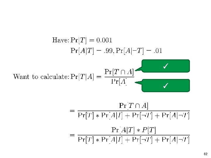
Formalization • 1 is terrorists, and we have their pictures. Thus the base rate of terrorists is 1/1000. P[T] = 0. 001 • 99/100 times when someone is a terrorist there is an alarm. P[A|T] =. 99 • For every 100 good guys, the alarm only goes off once. P[A | not T] =. 01 City • Want to know P[T|A] (this times 10) 77

Intuition: Given 999 good guys, we have 999*. 01 ≈ 9 -10 false alarms • 1 is terrorists, and we have their pictures. Thus the base rate of terrorists is 1/1000. P[T] = 0. 001 • 99/100 times when someone is a terrorist there is an alarm. P[A|T] =. 99 • For every 100 good guys, the alarm only goes off once. P[A | not T] =. 01 City False alarms (this times 10) • Want to know P[T|A] 78

Unknown 79
![Recall to get Pr[A] Fact: Proof: 80](http://slidetodoc.com/presentation_image_h/85c0fe5951ec91fed593439459e96901/image-80.jpg "Recall to get Pr[A] Fact: Proof: 80")
Recall to get Pr[A] Fact: Proof: 80
![. . and to get Pr[A∩ I] Fact: Proof: 81](http://slidetodoc.com/presentation_image_h/85c0fe5951ec91fed593439459e96901/image-81.jpg ". . and to get Pr[A∩ I] Fact: Proof: 81")
. . and to get Pr[A∩ I] Fact: Proof: 81

83
 Plot true positive vs. false positive for a")
Visualization: ROC (Receiver Operating Characteristics Curve) Plot true positive vs. false positive for a binary classifier at various threshold settings 84

For IDS Let 70% detection requires FP < 1/100, 000 True positives – I be an intrusion, A an alert from the IDS – 1, 000 msgs per day processed – 2 attacks per day – 10 attacks per message From Axelsson, RAID 99 80% detection generates 40% FP False positives 85

Why is anomaly detection hard Think in terms of ROC curves and the Base Rate fallacy. – Are real things rare? If so, hard to learn – Are real things common? If so, probably ok. 86

Conclusion • Firewalls – 3 types: Packet filtering, Stateful, and Application – Placement and DMZ • IDS – Anomaly vs. policy-based detection • Detection theory – Base rate fallacy 87
- Slides: 87