Finite State Machines 3 15 121 Introduction to

Finite State Machines 3 15 -121 Introduction to Data Structures 1

Notes taken with modifications from “Introduction to Automata Theory, Languages, and Computation” by John Hopcroft and Jeffrey Ullman, 1979 15 -121 Introduction to Data Structures 2

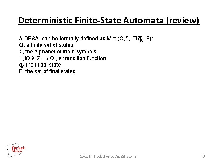
Deterministic Finite-State Automata (review) A DFSA can be formally defined as M = (Q, Σ, �� , q 0, F): Q, a finite set of states Σ, the alphabet of input symbols �� , Q X Σ → Q , a transition function q 0, the initial state F, the set of final states 15 -121 Introduction to Data Structures 3

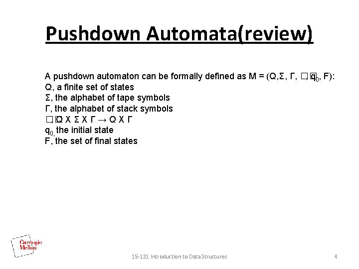
Pushdown Automata(review) A pushdown automaton can be formally defined as M = (Q, Σ, Γ, �� , q 0, F): Q, a finite set of states Σ, the alphabet of tape symbols Γ, the alphabet of stack symbols �� , QXΣXΓ→QXΓ q 0, the initial state F, the set of final states 15 -121 Introduction to Data Structures 4

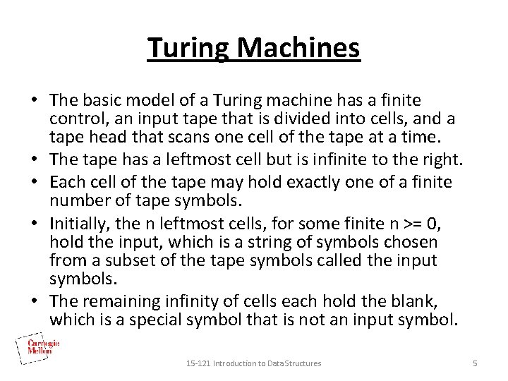
Turing Machines • The basic model of a Turing machine has a finite control, an input tape that is divided into cells, and a tape head that scans one cell of the tape at a time. • The tape has a leftmost cell but is infinite to the right. • Each cell of the tape may hold exactly one of a finite number of tape symbols. • Initially, the n leftmost cells, for some finite n >= 0, hold the input, which is a string of symbols chosen from a subset of the tape symbols called the input symbols. • The remaining infinity of cells each hold the blank, which is a special symbol that is not an input symbol. 15 -121 Introduction to Data Structures 5

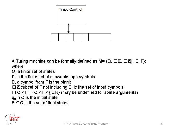
A Turing machine can be formally defined as M= (Q, �� , Γ, �� , q 0 , B, F): where Q, a finite set of states Γ, is the finite set of allowable tape symbols B, a symbol from Γ is the blank �� , a subset of Γ not including B, is the set of input symbols �� , Q x Γ → Q x Γ x { L, R} (may be undefined for some arguments) q 0 in Q is the initial state F ⊆Q is the set of final states 15 -121 Introduction to Data Structures 6

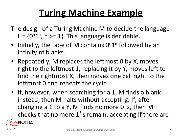
Turing Machine Example The design of a Turing Machine M to decide the language L = {0 n 1 n, n >= 1}. This language is decidable. • Initially, the tape of M contains 0 n 1 n followed by an infinity of blanks. • Repeatedly, M replaces the leftmost 0 by X, moves right to the leftmost 1, replacing it by Y, moves left to find the rightmost X, then moves one cell right to the leftmost 0 and repeats the cycle. • If, however, when searching for a 1, M finds a blank instead, then M halts without accepting. If, after changing a 1 to a Y, M finds no more 0’s, then M checks that no more 1’s remain, accepting if there are none. 15 -121 Introduction to Data Structures 7

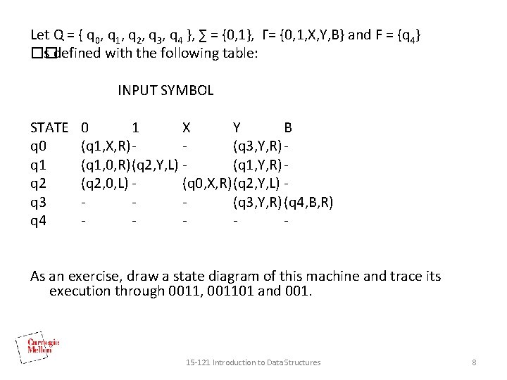
Let Q = { q 0, q 1, q 2, q 3, q 4 }, ∑ = {0, 1}, Γ= {0, 1, X, Y, B} and F = {q 4} �� is defined with the following table: INPUT SYMBOL STATE q 0 q 1 q 2 q 3 q 4 0 1 X Y B (q 1, X, R)(q 3, Y, R) (q 1, 0, R)(q 2, Y, L) (q 1, Y, R) (q 2, 0, L) (q 0, X, R)(q 2, Y, L) (q 3, Y, R) (q 4, B, R) - As an exercise, draw a state diagram of this machine and trace its execution through 0011, 001101 and 001. 15 -121 Introduction to Data Structures 8

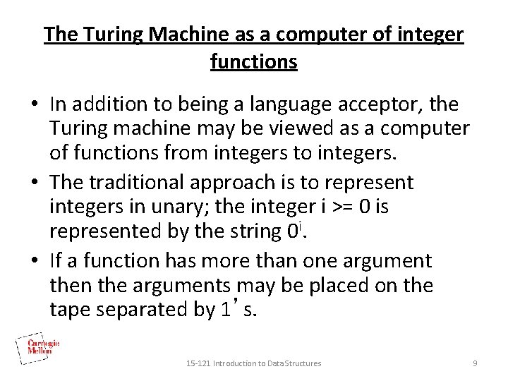
The Turing Machine as a computer of integer functions • In addition to being a language acceptor, the Turing machine may be viewed as a computer of functions from integers to integers. • The traditional approach is to represent integers in unary; the integer i >= 0 is represented by the string 0 i. • If a function has more than one argument then the arguments may be placed on the tape separated by 1’s. 15 -121 Introduction to Data Structures 9

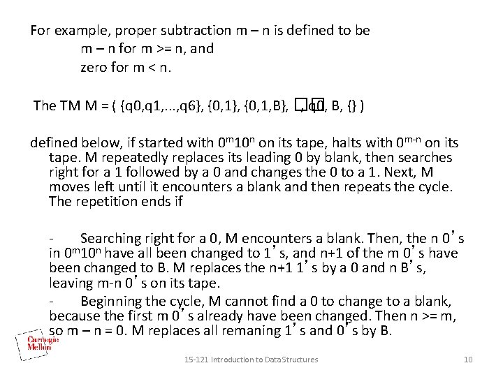
For example, proper subtraction m – n is defined to be m – n for m >= n, and zero for m < n. The TM M = ( {q 0, q 1, . . . , q 6}, {0, 1, B}, �� , q 0, B, {} ) defined below, if started with 0 m 10 n on its tape, halts with 0 m-n on its tape. M repeatedly replaces its leading 0 by blank, then searches right for a 1 followed by a 0 and changes the 0 to a 1. Next, M moves left until it encounters a blank and then repeats the cycle. The repetition ends if Searching right for a 0, M encounters a blank. Then, the n 0’s m in 0 10 n have all been changed to 1’s, and n+1 of the m 0’s have been changed to B. M replaces the n+1 1’s by a 0 and n B’s, leaving m-n 0’s on its tape. Beginning the cycle, M cannot find a 0 to change to a blank, because the first m 0’s already have been changed. Then n >= m, so m – n = 0. M replaces all remaning 1’s and 0’s by B. 15 -121 Introduction to Data Structures 10

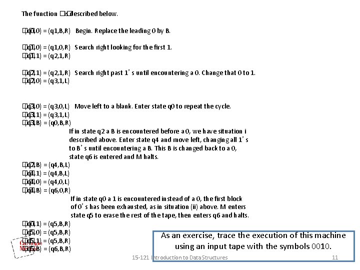
The function �� is described below. �� (q 0, 0) = (q 1, B, R) Begin. Replace the leading 0 by B. �� (q 1, 0) = (q 1, 0, R) Search right looking for the first 1. �� (q 1, 1) = (q 2, 1, R) �� (q 2, 1) = (q 2, 1, R) Search right past 1’s until encountering a 0. Change that 0 to 1. �� (q 2, 0) = (q 3, 1, L) �� (q 3, 0) = (q 3, 0, L) Move left to a blank. Enter state q 0 to repeat the cycle. �� (q 3, 1) = (q 3, 1, L) �� (q 3, B) = (q 0, B, R) If in state q 2 a B is encountered before a 0, we have situation i described above. Enter state q 4 and move left, changing all 1’s to B’s until encountering a B. This B is changed back to a 0, state q 6 is entered and M halts. �� (q 2, B) = (q 4, B, L) �� (q 4, 1) = (q 4, B, L) �� (q 4, 0) = (q 4, 0, L) �� (q 4, B) = (q 6, 0, R) If in state q 0 a 1 is encountered instead of a 0, the first block of 0’s has been exhausted, as in situation (ii) above. M enters state q 5 to erase the rest of the tape, then enters q 6 and halts. �� (q 0, 1) = (q 5, B, R) �� (q 5, 0) = (q 5, B, R) As an exercise, trace the execution of this machine �� (q 5, 1) = (q 5, B, R) using an input tape with the symbols 0010. �� (q 5, B) = (q 6, B, R). 15 -121 Introduction to Data Structures 11

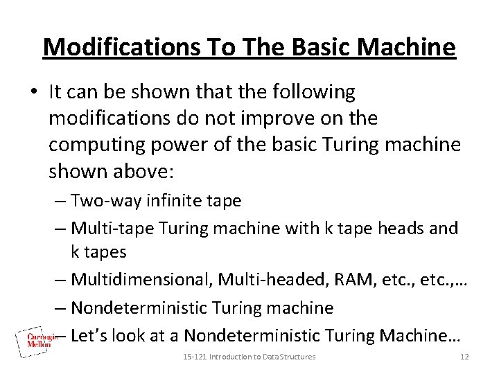
Modifications To The Basic Machine • It can be shown that the following modifications do not improve on the computing power of the basic Turing machine shown above: – Two-way infinite tape – Multi-tape Turing machine with k tape heads and k tapes – Multidimensional, Multi-headed, RAM, etc. , … – Nondeterministic Turing machine – Let’s look at a Nondeterministic Turing Machine… 15 -121 Introduction to Data Structures 12

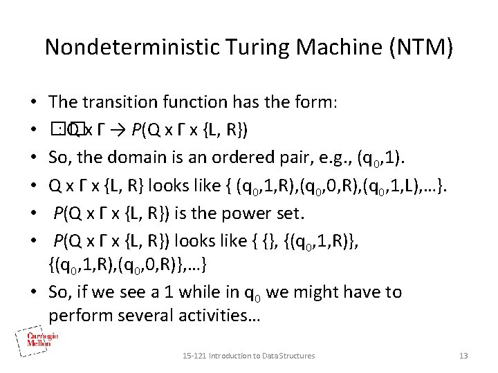
Nondeterministic Turing Machine (NTM) The transition function has the form: �� : Q x Γ → Ρ(Q x Γ x {L, R}) So, the domain is an ordered pair, e. g. , (q 0, 1). Q x Γ x {L, R} looks like { (q 0, 1, R), (q 0, 0, R), (q 0, 1, L), …}. Ρ(Q x Γ x {L, R}) is the power set. Ρ(Q x Γ x {L, R}) looks like { {}, {(q 0, 1, R), (q 0, 0, R)}, …} • So, if we see a 1 while in q 0 we might have to perform several activities… • • • 15 -121 Introduction to Data Structures 13

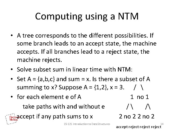
Computing using a NTM • A tree corresponds to the different possibilities. If some branch leads to an accept state, the machine accepts. If all branches lead to a reject state, the machine rejects. • Solve subset sum in linear time with NTM: • Set A = {a, b, c} and sum = x. Is there a subset of A summing to x? Suppose A = {1, 2}, x = 3. / • for each element e of A 1 no 1 take paths with and without e / / accept if any path sums to x 2 no 2 15 -121 Introduction to Data Structures 14 accept reject

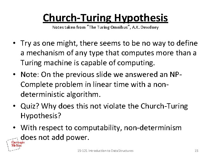
Church-Turing Hypothesis Notes taken from “The Turing Omnibus”, A. K. Dewdney • Try as one might, there seems to be no way to define a mechanism of any type that computes more than a Turing machine is capable of computing. • Note: On the previous slide we answered an NPComplete problem in linear time with a nondeterministic algorithm. • Quiz? Why does this not violate the Church-Turing Hypothesis? • With respect to computability, non-determinism does not add power. 15 -121 Introduction to Data Structures 15

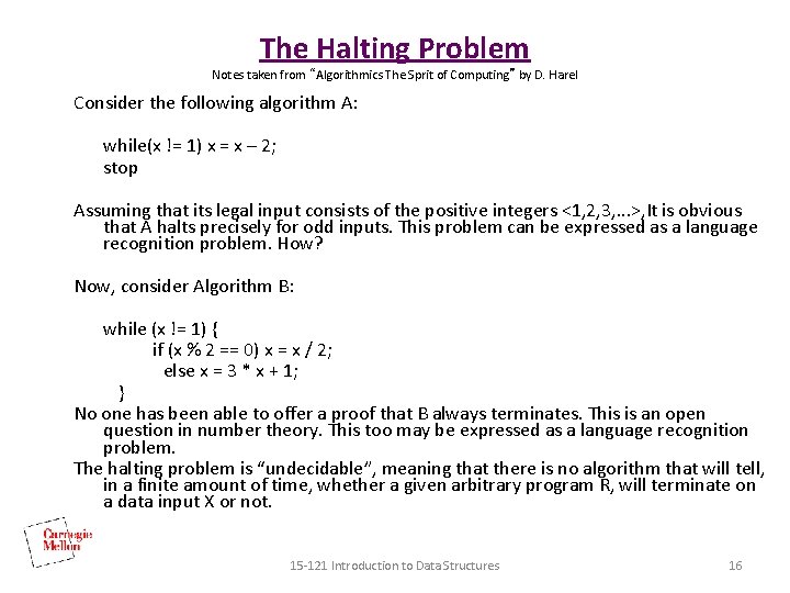
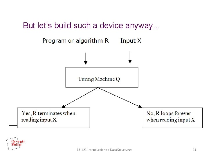
The Halting Problem Notes taken from “Algorithmics The Sprit of Computing” by D. Harel Consider the following algorithm A: while(x != 1) x = x – 2; stop Assuming that its legal input consists of the positive integers <1, 2, 3, . . . >, It is obvious that A halts precisely for odd inputs. This problem can be expressed as a language recognition problem. How? Now, consider Algorithm B: while (x != 1) { if (x % 2 == 0) x = x / 2; else x = 3 * x + 1; } No one has been able to offer a proof that B always terminates. This is an open question in number theory. This too may be expressed as a language recognition problem. The halting problem is “undecidable”, meaning that there is no algorithm that will tell, in a finite amount of time, whether a given arbitrary program R, will terminate on a data input X or not. 15 -121 Introduction to Data Structures 16

But let’s build such a device anyway… 15 -121 Introduction to Data Structures 17

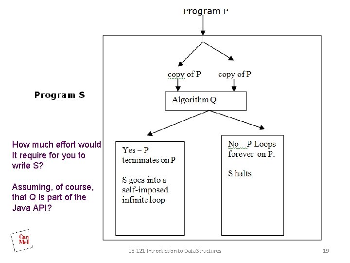
And let’s use it as a subroutine… • Build a new program S that uses Q in the following way. • S first makes a copy of its input. It then passes both copies (one as a program and another as its input) to Q. • Q makes its decision as before and gives its result back to S. • S halts if Q reports that Q’s input would loop forever. • S itself loops forever if Q reports that Q’s input terminates. 15 -121 Introduction to Data Structures 18

How much effort would It require for you to write S? Assuming, of course, that Q is part of the Java API? 15 -121 Introduction to Data Structures 19

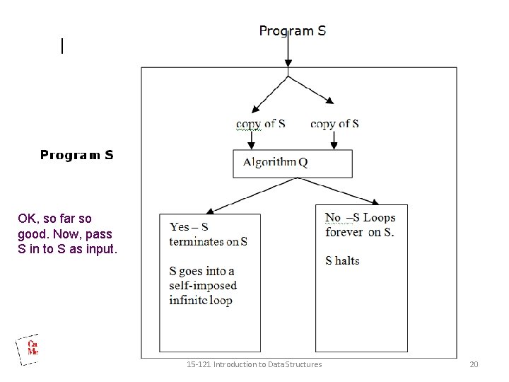
OK, so far so good. Now, pass S in to S as input. 15 -121 Introduction to Data Structures 20

• The existence of S leads to a logical contradiction. If S terminates when reading itself as input then Q reports this fact and S starts looping and never terminates. If S loops forever when reading itself as input then Q reports this to be the case and S terminates. • The construction of S seems to be reasonable in many respects. It makes a copy of its input. It calls a function called Q. It gets a result back and uses that result to decide whether or not to loop (a bit strange but easy to program). So, the problem must be with Q. Its existence implies a contradiction. So, Q does not exist. The halting problem is undecidable. 15 -121 Introduction to Data Structures 21

Example: Malware Detection • Shown to be undecidable • Do we give up? • No – monitoring output of processes can still be fruitful 15 -121 Introduction to Data Structures 22

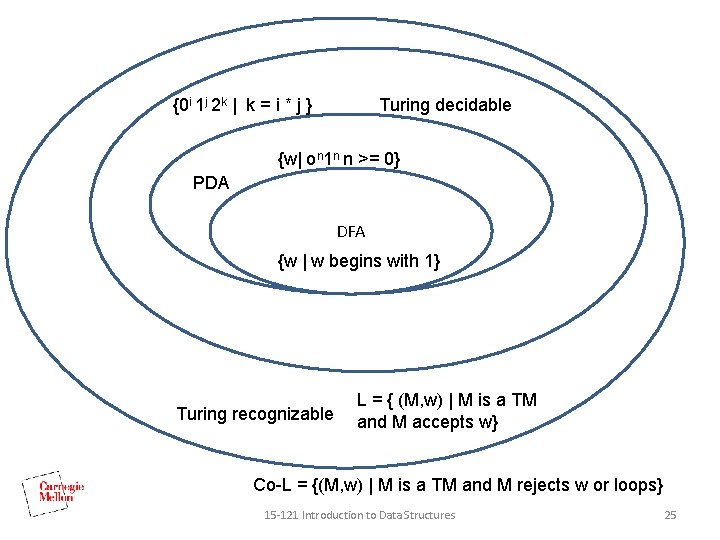
Terminology: Recursive and Recursively Enumerable notes from Wikipedia • A formal language is recursive if there exists a Turing machine which halts for every given input and always either accepts or rejects candidate strings. This is also called a decidable language. • A recursively enumerable language requires that some Turing machine halts and accepts when presented with a string in the language. It may either halt and reject or loop forever when presented with a string not in the language. A machine can recognize the language. • The set of halting program integer pairs is in R. E. but is not recursive. We can’t decide it but we can recognize it. • All recursive (decidable) languages are recursively enumerable. 15 -121 Introduction to Data Structures 23

Recursive and Recursively Enumerable • The set of halting program integer pairs is in R. E. but is not recursive. • Are there any languages that are not recursively enumerable? • Yes. Let L be { w = (program p, integer i) | p loops forever on i}. • L is not recursively enumerable. • We can’t even recognize L. • The set of languages is bigger than the set of Turing machines. 15 -121 Introduction to Data Structures 24

{0 i 1 j 2 k | k = i * j } Turing decidable {w| on 1 n n >= 0} PDA DFA {w | w begins with 1} Turing recognizable L = { (M, w) | M is a TM and M accepts w} Co-L = {(M, w) | M is a TM and M rejects w or loops} 15 -121 Introduction to Data Structures 25

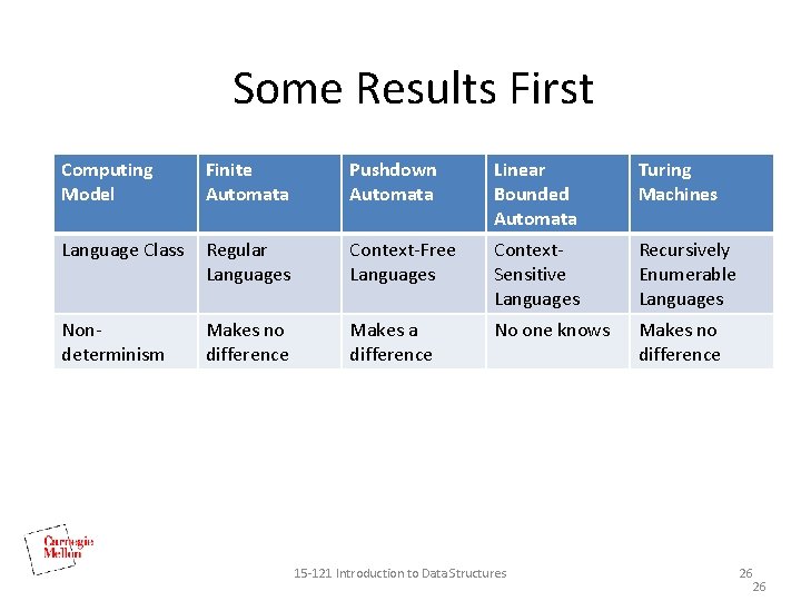
Some Results First Computing Model Finite Automata Pushdown Automata Linear Bounded Automata Turing Machines Language Class Regular Languages Context-Free Languages Context. Sensitive Languages Recursively Enumerable Languages Nondeterminism Makes no difference Makes a difference No one knows Makes no difference 15 -121 Introduction to Data Structures 26 26