Finite Potential Well The potential energy is zero
 = 0) when the")
 = U . I 0")
 = 0 • This is the same situation")


 Outside the potential • well, classical")
 |2 The probability")

- Slides: 10
Finite Potential Well The potential energy is zero • (U(x) = 0) when the particle is 0 < x < L (Region II) The energy has a finite value • (U(x) = U) outside this region, i. e. for x < 0 and x > L (Regions I and III) We also assume that energy • of the particle, E, is less than the “height” of the barrier, i. e. E < U
Finite Potential Well Schrödinger Equation x < 0; U(x) = U . I 0 < x < L; U(x) = 0 . II x > L; U(x) = 0. III
Finite Potential Well: Region II U(x) = 0 • This is the same situation as – previously for infinite potential well The allowed wave functions – are sinusoidal The general solution is • ψII(x) = F sin kx + G cos kx where F and G are constants – The boundary • conditions , however, no longer require that ψ(x) be zero at the ends of the well
Finite Potential Well: Regions I and III The Schrödinger equation for these regions is • It can be re-written as • The general solution of this equation is • ψ(x) = Ae. Cx + Be-Cx A and B are constants –
Finite Potential Well – Regions I and III Requiring that wavefunction was finite at x • ∞ and x - ∞, we can show that In region I, B = 0, and ψI(x) = Ae. Cx • This is necessary to avoid an infinite value for – ψ(x) for large negative values of x In region III, A = 0, and ψIII(x) = Be-Cx • This is necessary to avoid an infinite value for – ψ(x) for large positive values of x
Finite Potential Well The wavefunction and its derivative must be single-valued • for all x There are only two points where the wavefunction might have more – than one value: x = 0 and x = L Thus, we have to equate “parts” of the wavefunction and its derivative at x = 0, L This, together with – normalization condition, allows to determine the constants and the equation for energy of the particle •
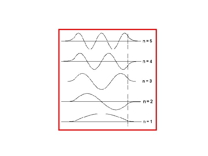
Finite Potential Well Graphical Results for ψ (x) Outside the potential • well, classical physics forbids the presence of the particle Quantum mechanics • shows the wave function decays exponentially to approach zero
Finite Potential Well Graphical Results for Probability Density, | ψ (x) |2 The probability densities • for the lowest three states are shown The functions are smooth • at the boundaries Outside the box, the • probability to find the particle decreases exponentially, but it is not zero!
Fig 3. 15 From Principles of Electronic Materials and Devices, Third Edition, S. O. Kasap (© Mc. Graw-Hill, 2005)