Finite Mixture Model With Application in Latent Trajectories

Finite Mixture Model: With Application in Latent Trajectories Ying Lu prepared for STAT 321 class presentation 10/23/2021 1

Outline • Introduction to Finite Mixture Model – Model formulation – Model estimation • Estimating mixing distribution • Incomplete-data and EM algorithm • Identifiability of mixture distributions • Testing the number of clusters 10/23/2021 2

Outline • Modeling Uncertainty in Latent Class Membership: A case study in Criminology (Roeder, Lynch and Nagin, 1999) 10/23/2021 3

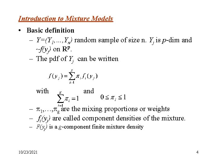
Introduction to Mixture Models • Basic definition – Y=(Y 1, …, Yn) random sample of size n. Yj is p-dim and ~f(yj) on Rp. – The pdf of Yj can be written with and – 1, …, g are the mixing proportions or weights – fi(yj) are called component densities of the mixture. – F(yj) is a g-component finite mixture density 10/23/2021 4

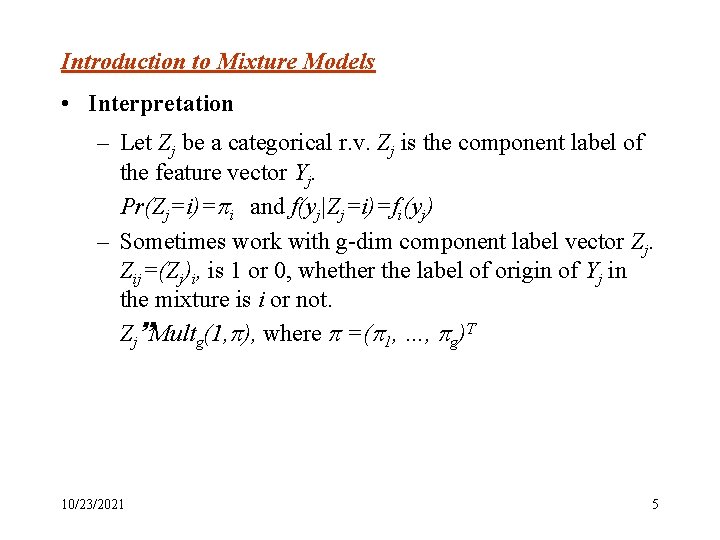
Introduction to Mixture Models • Interpretation – Let Zj be a categorical r. v. Zj is the component label of the feature vector Yj. Pr(Zj=i)= i and f(yj|Zj=i)=fi(yj) – Sometimes work with g-dim component label vector Zj. Zij=(Zj)i, is 1 or 0, whether the label of origin of Yj in the mixture is i or not. Zj Multg(1, ), where =( 1, …, g)T 10/23/2021 5

Introduction to Mixture Models An interesting niche between parametric and nonparametric approaches to statistical estimation and modeling heterogeneity. A semi-parametric compromise between – a fully parametric model with single parametric family (g=1); – and a non-parametric model by the kernel estimation (g=n). 10/23/2021 6

Introduction to Mixture Models • When applicable? Assume that Yj is drawn from a population G which consist of g subgroups, G 1, …, Gg in proportions 1, . . . g. Two scenarios: – Groups are known: two groups, with or without diseases, estimate disease prevalence. – Groups are unknown: more interesting. model-based approach to clustering. 10/23/2021 7

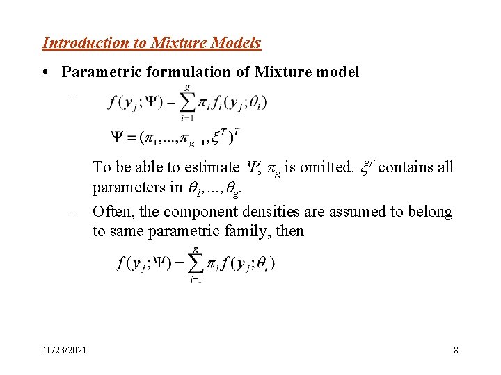
Introduction to Mixture Models • Parametric formulation of Mixture model – To be able to estimate , g is omitted. T contains all parameters in 1, …, g. – Often, the component densities are assumed to belong to same parametric family, then 10/23/2021 8

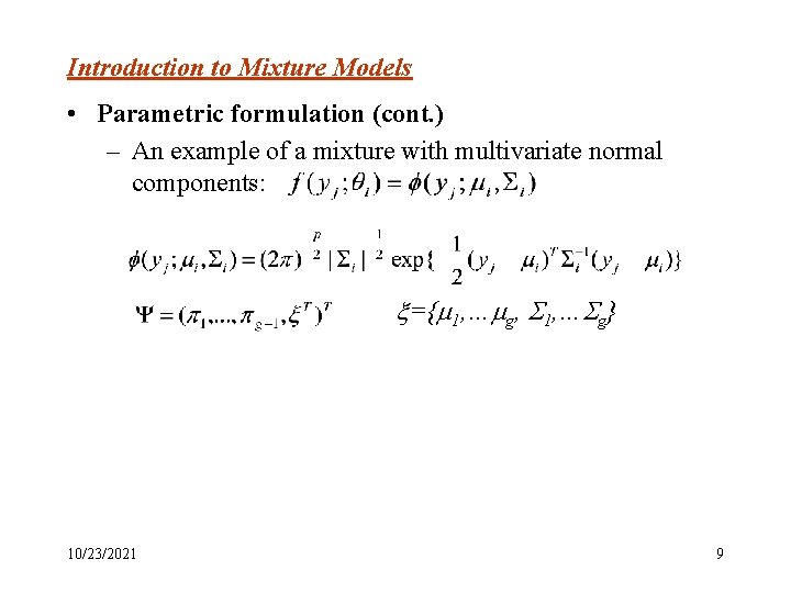
Introduction to Mixture Models • Parametric formulation (cont. ) – An example of a mixture with multivariate normal components: ={ 1, … g, 1, … g} 10/23/2021 9

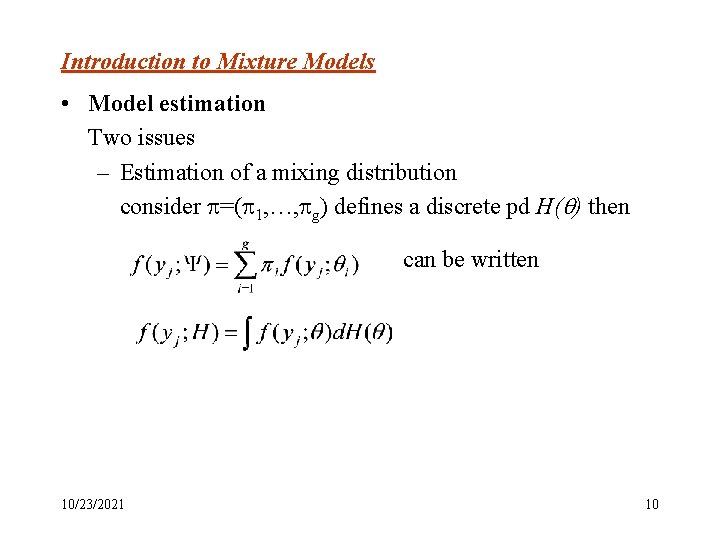
Introduction to Mixture Models • Model estimation Two issues – Estimation of a mixing distribution consider =( 1, …, g) defines a discrete pd H( ) then can be written 10/23/2021 10

Introduction to Mixture Models – Estimate mixing distribution (cont. ) On estimating H( ), Lindsay (1983) considered the “nonparametric” ML estimation of the mixing distribution H. He showed that finding the MLE involved a standard problem of convex optimization, In particular, it is possible to determine by evaluation of a simple gradient function how close a candidate estimator H* is to a ML solution H. 10/23/2021 11

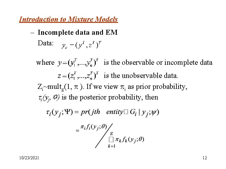
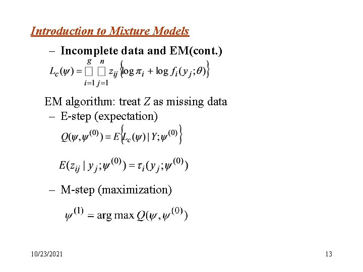
Introduction to Mixture Models – Incomplete data and EM Data: where is the observable or incomplete data is the unobservable data. Zi~multg(1, ). If we view i as prior probability, i(yj, ) is the posterior probability, then 10/23/2021 12

Introduction to Mixture Models – Incomplete data and EM(cont. ) EM algorithm: treat Z as missing data – E-step (expectation) – M-step (maximization) 10/23/2021 13

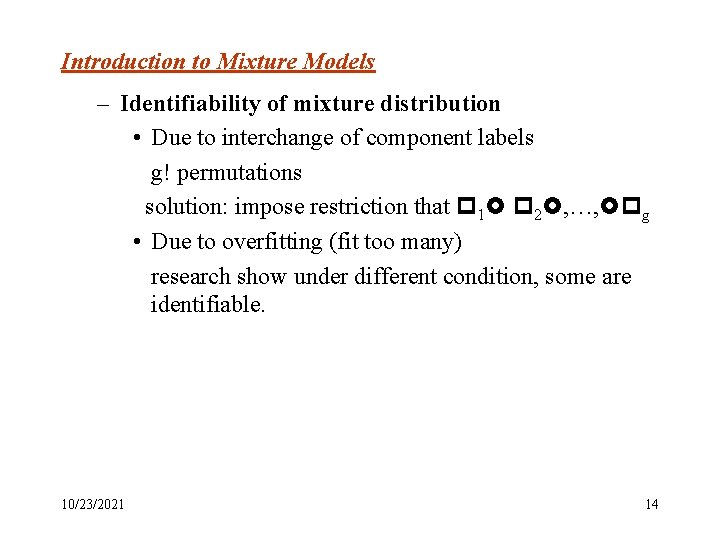
Introduction to Mixture Models – Identifiability of mixture distribution • Due to interchange of component labels g! permutations solution: impose restriction that 1 2 , …, g • Due to overfitting (fit too many) research show under different condition, some are identifiable. 10/23/2021 14

Introduction to Mixture Models – Test the number of components • LRT? sometimes, the regularity condition doesn’t hold asymptotic chi-squared distribution? • Various revised version of LRTs • Bootstrap method, need large K • Bayesian method, such as BIC 10/23/2021 15

Introduction to Mixture Models • Model estimation (cont. 4) Other attempts: – To minimize , the distance between the mixture distribution F and the empirical distribution function that places mass one at each data point yj (j=1, …n) 10/23/2021 16

Introduction to Mixture Models • Various applications – – – Mixture models with normal/non-normal components Mixture of factor analysis Mixture models for failure-time data Mixture analysis of directional data Hidden Markov Models • References Mc. Lachlan, G. and D. Peel. (2000) Finite Mixture Models Mc. Lachlan, G. and K. Basford (1988) …. 10/23/2021 17

Latent Trajectories Analysis: • Background Life-course and developmental theories of crime and deviance is to understand explain the evolution of such behaviors from childhood through adulthood. Such path of evolution is referred as criminal trajectory. • Moffitt’s theory(1993): – poor neurological development and poor parenting. – adolescent-limited offenders v. s. life-course-persistent offenders. • Objectives: – Is there such taxonomy? – What are the risk factors? 10/23/2021 18

Latent Trajectories Analysis: • Data – Cambridge Study of Delinquent Development: a prospective longitudinal survey of 403 males from London (1961 -1983) – Start from 8 years old, continued for 22 years till 30 years old. – Criminal involvement measured by convictions for criminal offenses. (36%, 4. 4!) – measurements of risk factors: • intelligence and attainment • antisocial family and parenting factors • hyperactivity, impulsivity, and attention deficits --daring 10/23/2021 19

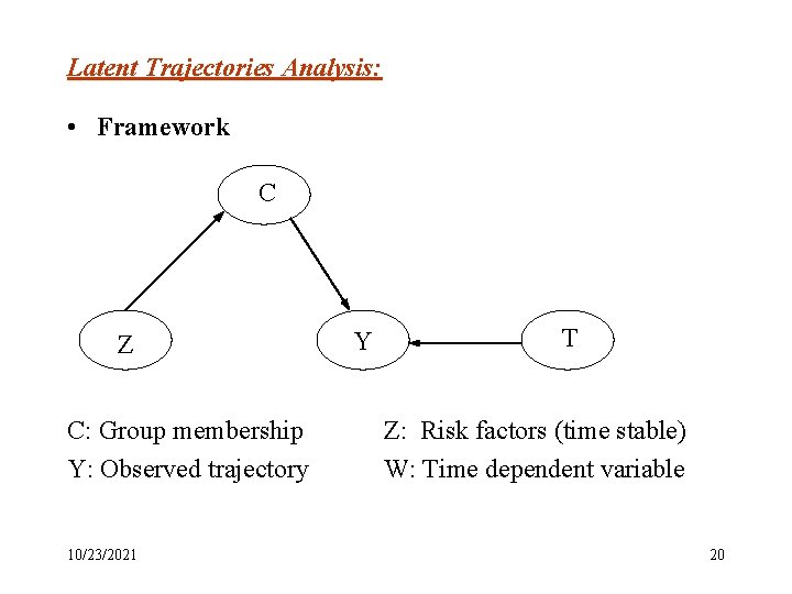
Latent Trajectories Analysis: • Framework C Z C: Group membership Y: Observed trajectory 10/23/2021 Y T Z: Risk factors (time stable) W: Time dependent variable 20

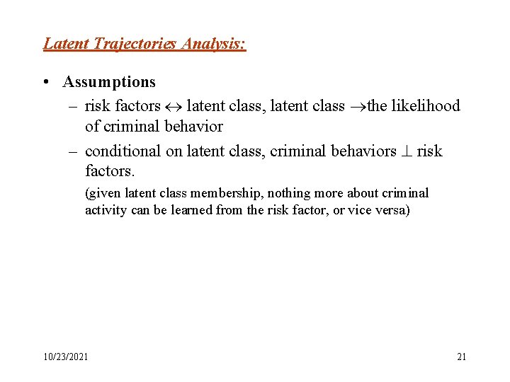
Latent Trajectories Analysis: • Assumptions – risk factors latent class, latent class the likelihood of criminal behavior – conditional on latent class, criminal behaviors risk factors. (given latent class membership, nothing more about criminal activity can be learned from the risk factor, or vice versa) 10/23/2021 21

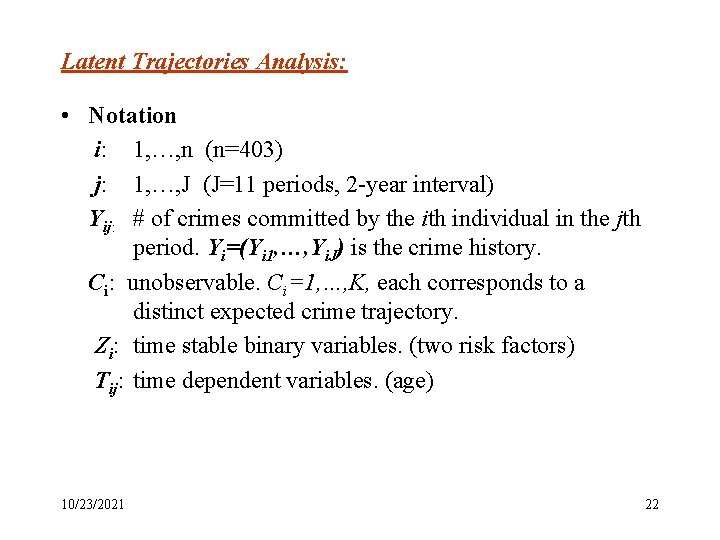
Latent Trajectories Analysis: • Notation i: 1, …, n (n=403) j: 1, …, J (J=11 periods, 2 -year interval) Yij: # of crimes committed by the ith individual in the jth period. Yi=(Yi 1, …, Yi. J) is the crime history. Ci: unobservable. Ci=1, …, K, each corresponds to a distinct expected crime trajectory. Zi: time stable binary variables. (two risk factors) Tij: time dependent variables. (age) 10/23/2021 22

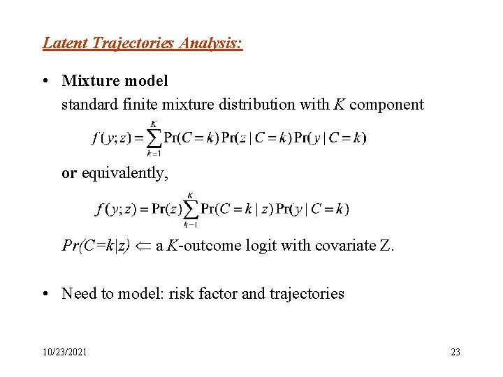
Latent Trajectories Analysis: • Mixture model standard finite mixture distribution with K component or equivalently, Pr(C=k|z) a K-outcome logit with covariate Z. • Need to model: risk factor and trajectories 10/23/2021 23

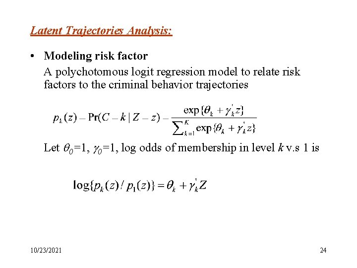
Latent Trajectories Analysis: • Modeling risk factor A polychotomous logit regression model to relate risk factors to the criminal behavior trajectories Let 0=1, log odds of membership in level k v. s 1 is 10/23/2021 24

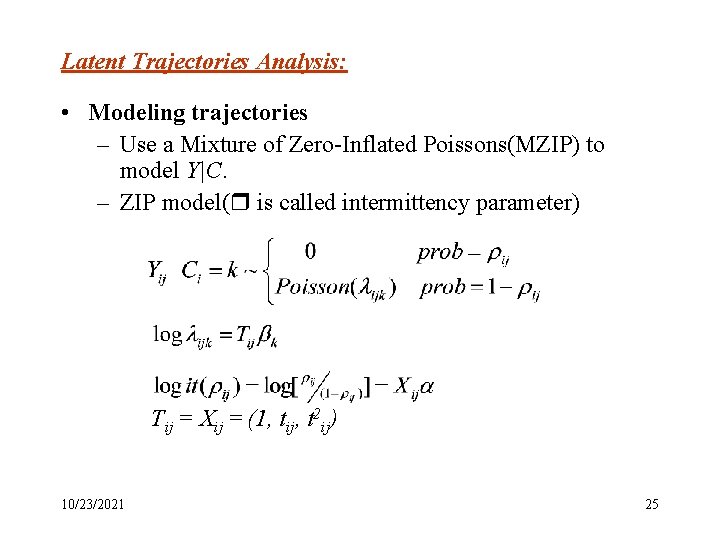
Latent Trajectories Analysis: • Modeling trajectories – Use a Mixture of Zero-Inflated Poissons(MZIP) to model Y|C. – ZIP model( is called intermittency parameter) Tij = Xij = (1, tij, t 2 ij) 10/23/2021 25

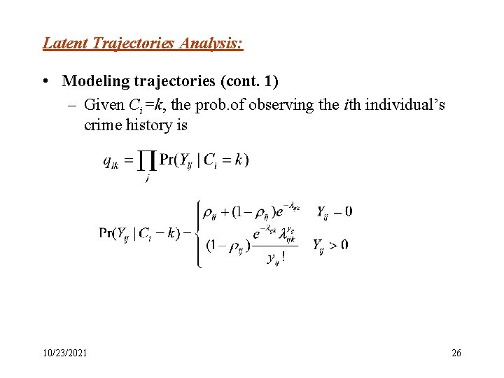
Latent Trajectories Analysis: • Modeling trajectories (cont. 1) – Given Ci=k, the prob. of observing the ith individual’s crime history is 10/23/2021 26

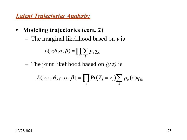
Latent Trajectories Analysis: • Modeling trajectories (cont. 2) – The marginal likelihood based on y is – The joint likelihood based on (y, z) is 10/23/2021 27

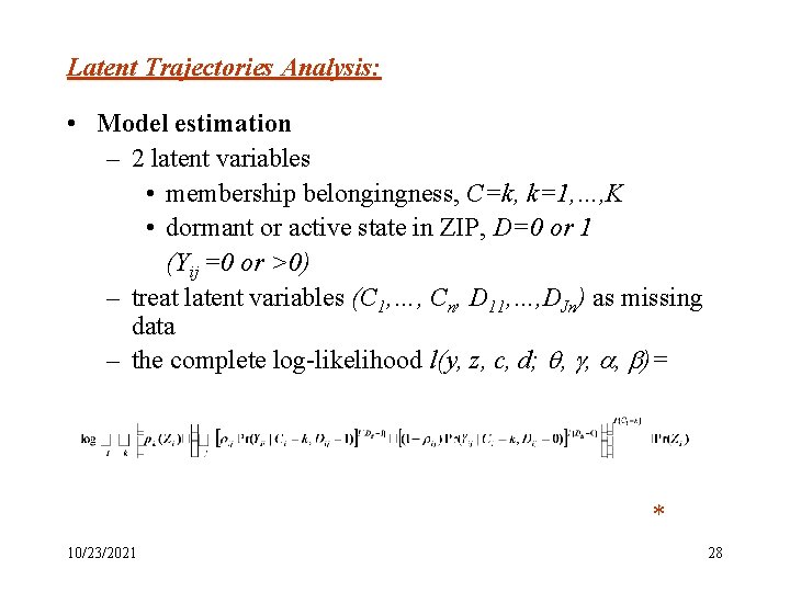
Latent Trajectories Analysis: • Model estimation – 2 latent variables • membership belongingness, C=k, k=1, …, K • dormant or active state in ZIP, D=0 or 1 (Yij =0 or >0) – treat latent variables (C 1, …, Cn, D 11, …, DJn) as missing data – the complete log-likelihood l(y, z, c, d; , , , )= * 10/23/2021 28

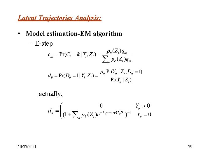
Latent Trajectories Analysis: • Model estimation-EM algorithm – E-step actually, 10/23/2021 29

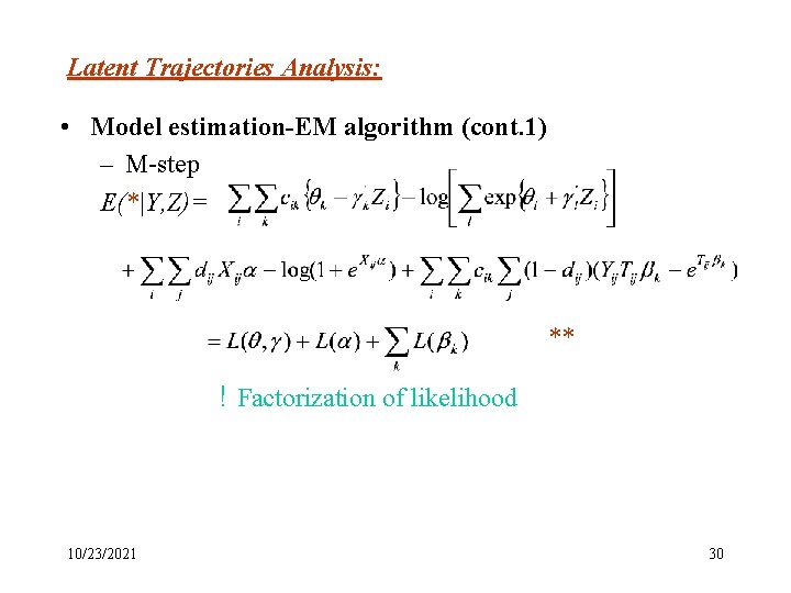
Latent Trajectories Analysis: • Model estimation-EM algorithm (cont. 1) – M-step E(*|Y, Z)= ** ! Factorization of likelihood 10/23/2021 30

Latent Trajectories Analysis: • Model estimation-EM algorithm (cont. 2) L( , ): weighted polychotomous logistic regression. [cij] L( ): weighted logistic regression. [ 1 -dij for Yij=0 dij, Yij=1] L( k): MZIP model. [ cik* (1 -dij)] 10/23/2021 31

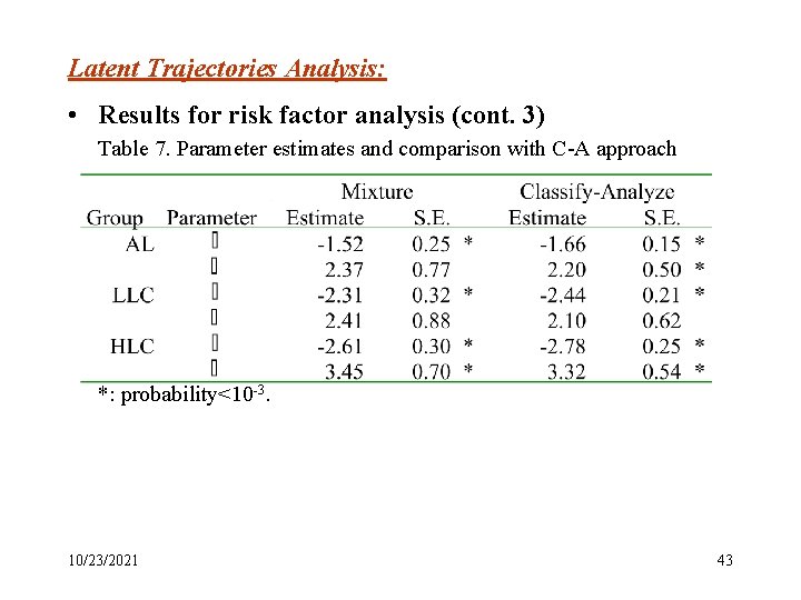
Latent Trajectories Analysis: • Risk Factor Analysis To identify risk factor for various criminal careers testing whether differs across latent groups – traditional approach: classify-analyze • classify by the largest posterior probability of membership, then analyze as if C was known • biased estimates. Exaggerate the certainty of group and inflate precision. – a likelihood ratio test based on the mixture model accounts for uncertainty in group membership 10/23/2021 32

Latent Trajectories Analysis: • Risk Factor Analysis (cont. ) Caveats – might not have asymptotic chi-squared distribution. – H 0 is often on the boundary of the parameter space. – Due to lack of identifiability, the degree of freedom is sometimes hard to count. – For this problem, H 0 is not on the boundary, and the difference in dimension of competing models is clearly defined. So 2 approximation will apply. 10/23/2021 33

Latent Trajectories Analysis: • Model Selection and BIC Use Bayesian Information Criterion to choose among different models Advantages: – It has good properties under weaker regularity condition than LRT (Keribin, 1998; Leroux, 1992; Roeder and Wasserman, 1997. ) – It is consistent even when the models are not nested (Nishii, 1988. ) 10/23/2021 34

Latent Trajectories Analysis: • Results Goal is to test: – whether the life-course-persistent and adolescent-limited trajectories are present in the data. – whethere is a distinctive etiology of the former group. Specifcally, an interaction between neurological deficits and poor child-rearing practices in heightening the probability of following a trajectory of chronic offending. 10/23/2021 35

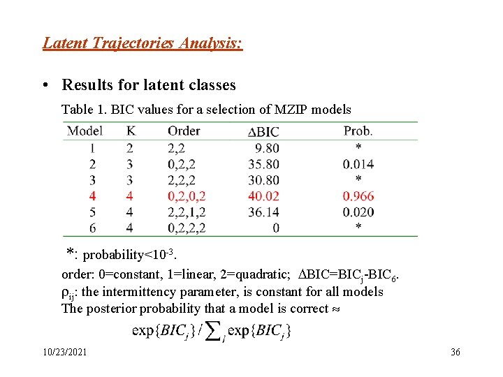
Latent Trajectories Analysis: • Results for latent classes Table 1. BIC values for a selection of MZIP models *: probability<10 -3. order: 0=constant, 1=linear, 2=quadratic; BIC=BICj-BIC 6. ij: the intermittency parameter, is constant for all models The posterior probability that a model is correct 10/23/2021 36

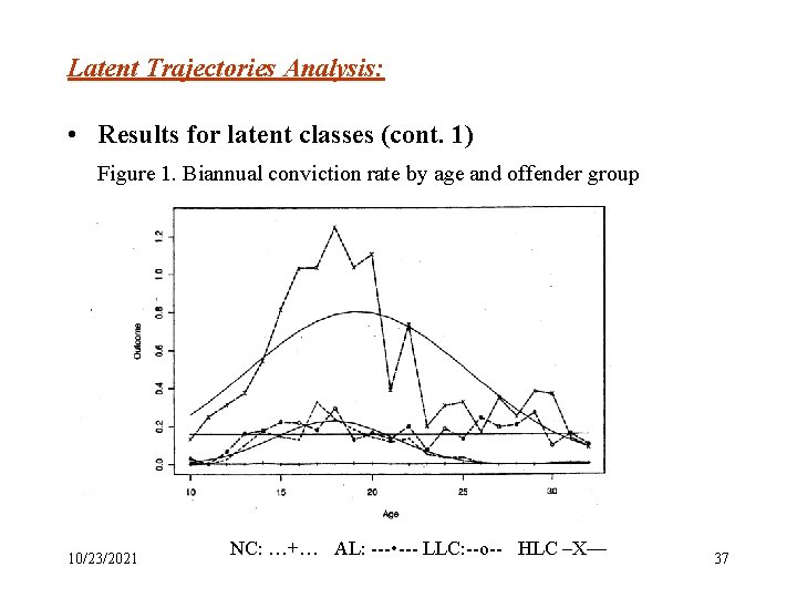
Latent Trajectories Analysis: • Results for latent classes (cont. 1) Figure 1. Biannual conviction rate by age and offender group 10/23/2021 NC: …+… AL: --- • --- LLC: --o-- HLC –X— 37

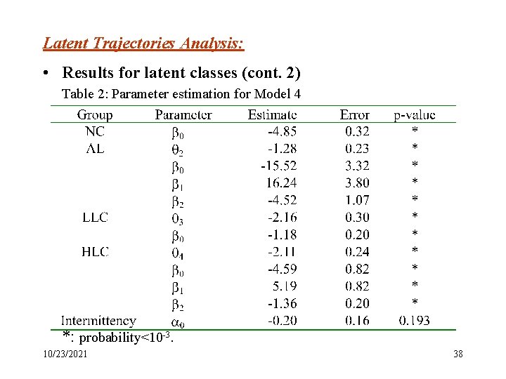
Latent Trajectories Analysis: • Results for latent classes (cont. 2) Table 2: Parameter estimation for Model 4 *: probability<10 -3. 10/23/2021 38

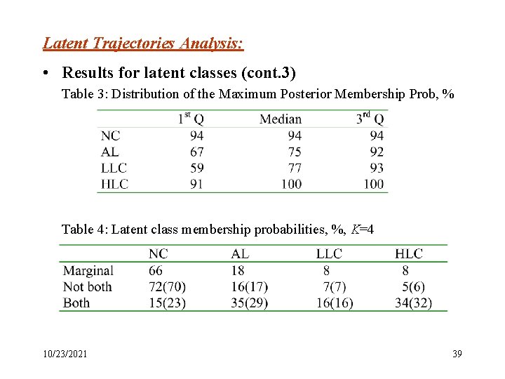
Latent Trajectories Analysis: • Results for latent classes (cont. 3) Table 3: Distribution of the Maximum Posterior Membership Prob, % Table 4: Latent class membership probabilities, %, K=4 10/23/2021 39

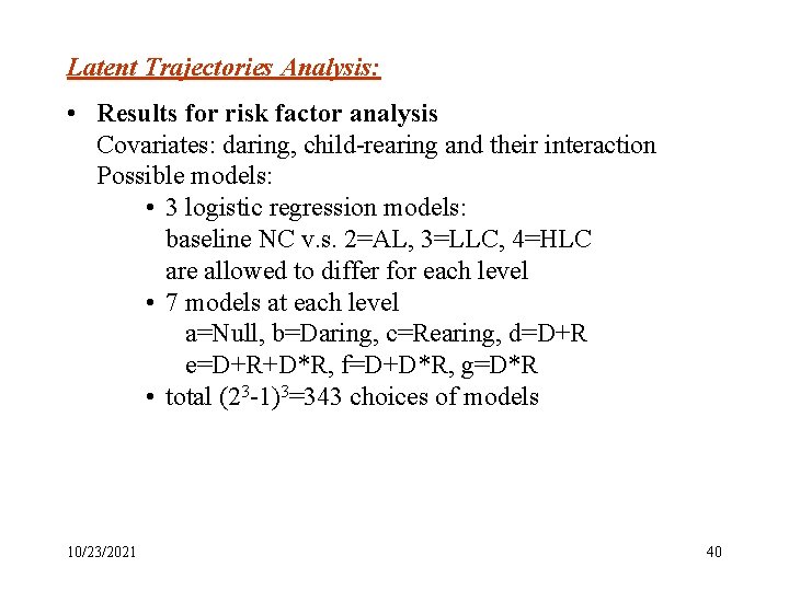
Latent Trajectories Analysis: • Results for risk factor analysis Covariates: daring, child-rearing and their interaction Possible models: • 3 logistic regression models: baseline NC v. s. 2=AL, 3=LLC, 4=HLC are allowed to differ for each level • 7 models at each level a=Null, b=Daring, c=Rearing, d=D+R e=D+R+D*R, f=D+D*R, g=D*R • total (23 -1)3=343 choices of models 10/23/2021 40

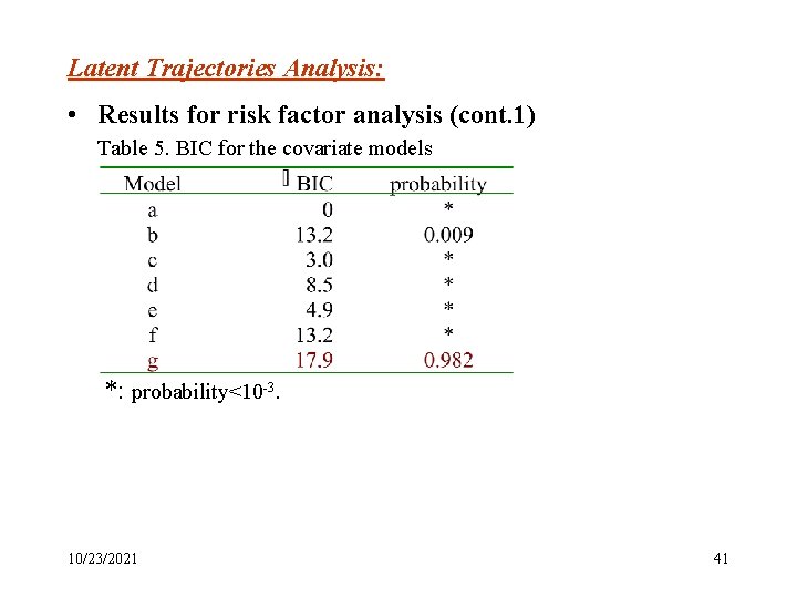
Latent Trajectories Analysis: • Results for risk factor analysis (cont. 1) Table 5. BIC for the covariate models *: probability<10 -3. 10/23/2021 41

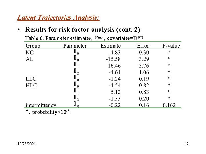
Latent Trajectories Analysis: • Results for risk factor analysis (cont. 2) Table 6. Parameter estimates, K=4, covariates=D*R *: probability<10 -3. 10/23/2021 42

Latent Trajectories Analysis: • Results for risk factor analysis (cont. 3) Table 7. Parameter estimates and comparison with C-A approach *: probability<10 -3. 10/23/2021 43

Latent Trajectories Analysis: • A SAS procedure for estimating developmental trajectories http: //lib. stat. cmu. edu/~bjones 10/23/2021 44

The end Thank 10/23/2021 You ! 45