FINITE FAULT MODELING OF STRONG GROUND MOTIONS USING

FINITE FAULT MODELING OF STRONG GROUND MOTIONS USING AN EMPIRICAL GREEN’S FUNCTION APPROACH Case Study: 26 September 1997, 09: 40 GMT, Mw= 6. 0 Colfiorito Earthquake (Italy) Laura Scognamiglio ISTANBUL JANUARY 2005

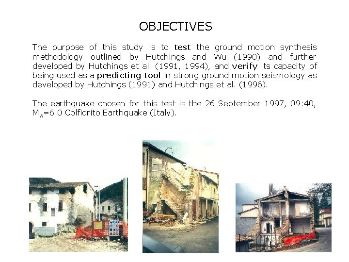
OBJECTIVES The purpose of this study is to test the ground motion synthesis methodology outlined by Hutchings and Wu (1990) and further developed by Hutchings et al. (1991, 1994), and verify its capacity of being used as a predicting tool in strong ground motion seismology as developed by Hutchings (1991) and Hutchings et al. (1996). The earthquake chosen for this test is the 26 September 1997, 09: 40, Mw=6. 0 Colfiorito Earthquake (Italy).

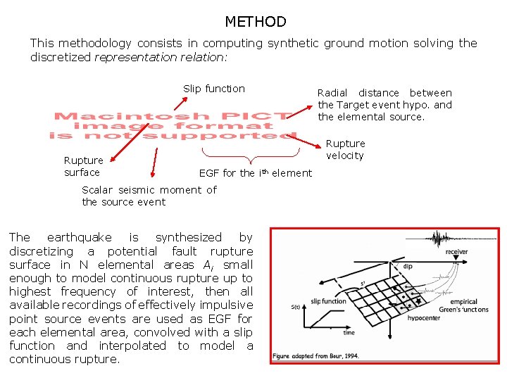
METHOD This methodology consists in computing synthetic ground motion solving the discretized representation relation: Slip function Rupture surface Radial distance between the Target event hypo. and the elemental source. Rupture velocity EGF for the ith element Scalar seismic moment of the source event The earthquake is synthesized by discretizing a potential fault rupture surface in N elemental areas Ai small enough to model continuous rupture up to highest frequency of interest, then all available recordings of effectively impulsive point source events are used as EGF for each elemental area, convolved with a slip function and interpolated to model a continuous rupture.

COOK BOOK: how computing synthetic seismograms with EGF The FIRST STEP consists in selecting a data-base of small earthquakes to be used as EGF. These events need to be generated by the same fault of the target event and to have same focal mechanism. Seismic moment and corner frequency of the events should be evaluated if not available. The SECOND STEP consists in constructing the rupture scenarios for the evaluation of the synthetic seismograms. These scenarios consist in a preferred number of faulting model defined by: strike, dip, slip vector, rupture area, rupture and healing velocity (rise times), roughness, hypocenter, and number and location of large asperities. Moment remains fixed. The parameters are varied about a preferred value and selected by a Monte Carlo pick using a triangular distribution.

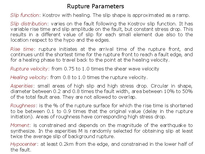
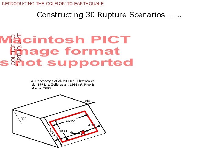
Rupture Parameters Slip function: Kostrov with healing. The slip shape is approximated as a ramp. Slip distribution: varies on the fault following the Kostrov slip function. It has variable rise time and slip amplitude on the fault, but constant stress drop. This results in a different value of slip for each small element due also to the location respect to the hypo and the edges. Rise time: rupture initiates at the arrival time of the rupture front, and continues until the shortest time for the rupture front to reach a fault edge, and for a healing phase to travel back to the point at the healing velocity. Rupture velocity: from 0. 75 to 1. 0 times the shear wave velocity Healing velocity: from 0. 8 to 1. 0 times the rupture velocity. Asperities: small areas of high slip and high stress drop. Circular in shape, diameter between 0. 2 and 0. 8 times the fault width, area between 10% to 50% of the total fault area. They are not allowed to overlap. Roughness: is the % of the rupture surface for which the rise time is shortened to be between 0. 1 to 0. 9 times that the original value (delay in the rupture initiation). Areas of roughness have corresponding high stress drop. Moment: is constrained and depends on the magnitude of the earthquake to synthesize. In the asperities M is randomly selected for obtaining slip at least twice the average slip of background rupture. Hypocenter: at least 0. 2 km from the edge, and constrained in the lower half of the fault.

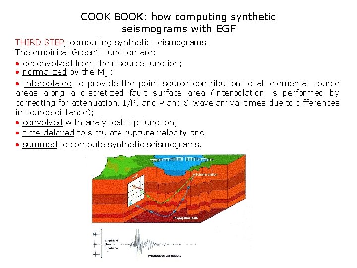
COOK BOOK: how computing synthetic seismograms with EGF THIRD STEP, computing synthetic seismograms. The empirical Green’s function are: • deconvolved from their source function; • normalized by the M 0 ; • interpolated to provide the point source contribution to all elemental source areas along a discretized fault surface area (interpolation is performed by correcting for attenuation, 1/R, and P and S-wave arrival times due to differences in source distance); • convolved with analytical slip function; • time delayed to simulate rupture velocity and • summed to compute synthetic seismograms.

DATA ANALYSES AND VALIDATION PROCEDURE 1. I have collected small earthquakes recorded by the same stations that recorded the Colfiorito Earthquake and occurred on the same fault; 2. I have evaluated seismic moment and corner frequency of these events; 3. I have constructed rupure scenarios to simulate the Colfiorito Earthquake rupture and I have calculate synthetic seismograms for each scenarios at each station. then, I have carried out a validation procedure based on two analyses: 4. a FORWARD MODELING analysis to find whether one of the synthetic seismograms obtained match the Colfiorito observed time histories; 5. a PREDICTION TOOL analysis to develop a range of possible ground motions and see if the actual ground motion recordings fall within the range predicted.

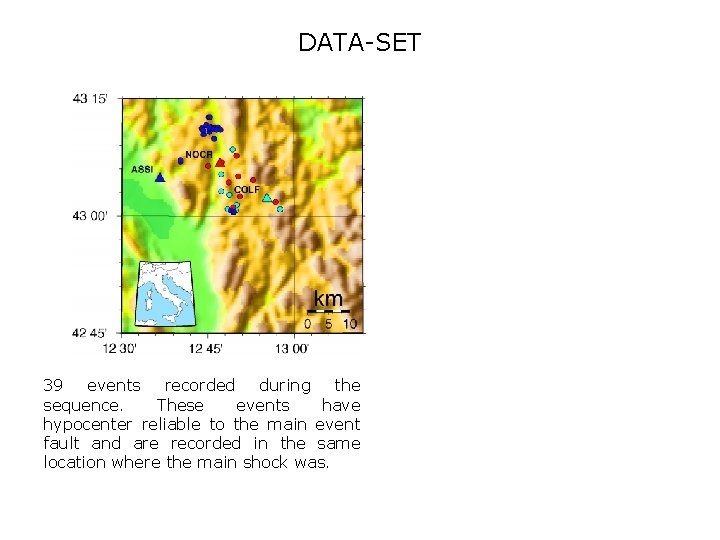
DATA-SET 39 events recorded during the sequence. These events have hypocenter reliable to the main event fault and are recorded in the same location where the main shock was.

REPRODUCING THE COLFIORITO EARTHQUAKE Constructing 30 Rupture Scenarios……. . a, Deschamps et al. 2000; b, Ekström et al. , 1998. c, Zollo et al. , 1999; d, Pino & Mazza, 2000. stkk dpp rec 22 dp pd is rh 22 rec 11 rh 11

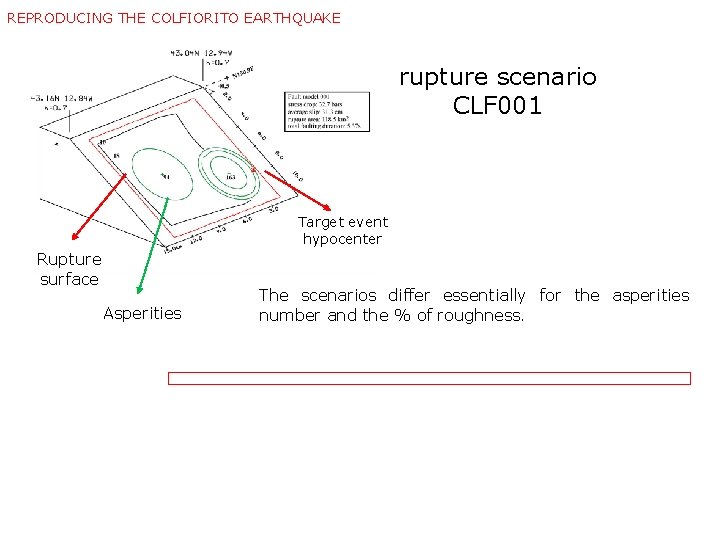
REPRODUCING THE COLFIORITO EARTHQUAKE rupture scenario CLF 001 Target event hypocenter Rupture surface Asperities The scenarios differ essentially for the asperities number and the % of roughness.

REPRODUCING THE COLFIORITO EARTHQUAKE COMPARISON IN THE SPECTRA RESPONSE DOMAIN For each model at each station, synthetic seismograms were calculated, then absolute acceleration response spectra (AAR) and the pseudo velocity response spectra (PSV) were evaluated and compared with the Colfiorito Earthquake response spectra.

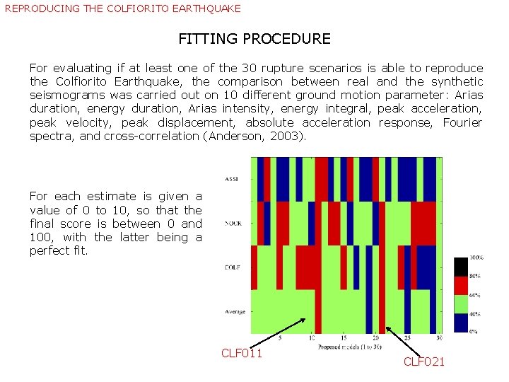
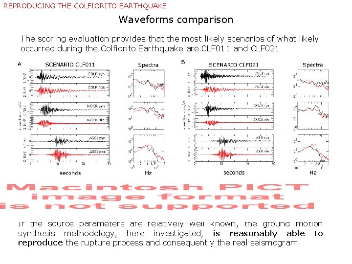
REPRODUCING THE COLFIORITO EARTHQUAKE FITTING PROCEDURE For evaluating if at least one of the 30 rupture scenarios is able to reproduce the Colfiorito Earthquake, the comparison between real and the synthetic seismograms was carried out on 10 different ground motion parameter: Arias duration, energy duration, Arias intensity, energy integral, peak acceleration, peak velocity, peak displacement, absolute acceleration response, Fourier spectra, and cross-correlation (Anderson, 2003). For each estimate is given a value of 0 to 10, so that the final score is between 0 and 100, with the latter being a perfect fit. CLF 011 CLF 021

REPRODUCING THE COLFIORITO EARTHQUAKE Waveforms comparison The scoring evaluation provides that the most likely scenarios of what likely occurred during the Colfiorito Earthquake are CLF 011 and CLF 021 If the source parameters are relatively well known, the ground motion synthesis methodology, here investigated, is reasonably able to reproduce the rupture process and consequently the real seismogram.

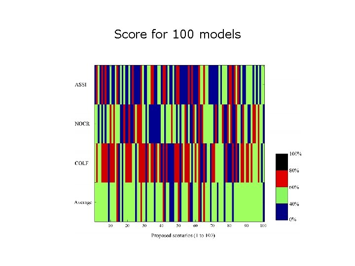
PREDICTING TOOL Strong Ground Motion “Prediction” Analysis I tried to establish the potential of this empirical Green’s function synthesis approach as a prediction tool in strong ground motion seismology. Constructing 100 rupture scenarios No previous information available on the Colfiorito Earthquake was used in calculating the rupture scenarios. I started from: • a normal fault in Apennine direction (NNW-SSE); • with dip coherent with the range showed by Umbria-Marche normal faults (Barchi et al. , 2000), • and fault dimension related with the magnitude of the earthquake to reproduce. THEN I EVALUATED SYNTHETIC SEISMOGRAMS FOR EACH MODEL AT EACH STATION AND I VERIFIED THAT COLFIORITO EARTHQUAKE FALLS IN BETWEEN THE RANGE PREDICTED.

PREDICTING TOOL COMPARISON IN THE SPECTRA RESPONSE DOMAIN Almost all the models are comprised between one standard deviation of the mean for the three stations. ASSI: AAR and PSV fit quite well the Colfiorito shape spectra in all the frequency band. Colfiorito earthquake lies close to the average curve. COLF and NOCR spectra show a quite good fit until 0. 3 -0. 4 s, for lower period the predicted ground motion overestimate the real one.

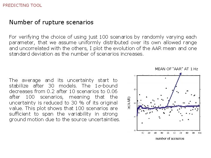
PREDICTING TOOL Number of rupture scenarios For verifying the choice of using just 100 scenarios by randomly varying each parameter, that we assume uniformly distributed over its own allowed range and uncorrelated with the others, I plot the evolution of the AAR mean and one standard deviation as the number of scenarios increases. MEAN OF “AAR” AT 1 Hz The average and its uncertainty start to stabilize after 30 models. The 1 -bound decreases from 0. 2 after 10 scenarios to 0. 06 after 100 scenarios, meaning that the uncertainty is reduced to 30 % of its original value. This plot shows that 100 scenarios are sufficient to span the variability in strong ground motion due to the source uncertainties.

RESULTS and CONCLUSIONS The purpose of this study was to test the ground motion synthesis methodology outlined by Hutchings and Wu (1990) for verifying its capability of being used as a predicting tool in strong ground motion seismology. The validation procedure was carried out on the 26 September 1997, Mw 6. 0 Colfiorito Earthquake. 1. The “forward modeling” analysis results demonstrate that this strong ground motion synthesis methodology is a technique capable, once the scenarios are well constrained by independent information, to reproduce reasonably well the observed records; 2. comparing the Colfiorito spectra (AAR and PSV) with spectra calculated from 100 rupture scenarios, constructed without including any knowledge of the source characteristics, emerges that it is possible to make reasonable strong ground motion “predictions” even without having a priori knowledge of the fault characteristics, by running enough models.

THE END!!!!

RESULTS…… Synthesis of Colfiorito Earthquake SPECTRA RESPONSE DOMAIN COMPARISON • Colfiorito response spectra fall inside the 30 AAR’s and PSV’s calculated at ASSI and COLF, showing the same amplitude of the average calculated for these synthetics; • synthetic spectra at NOCR, on average, overestimate the real ground motion. In the range of periods analyzed here, the latter follows the curve defined by the average minus one standard deviation; SCORING PROCEDURE • the quantitative matching evaluation shows that, in the thirty scenarios tried, two combinations of source parameters give a good fit for all the three stations (Models 011 and 021). Strong Ground Motion “Prediction” Analysis SPECTRA RESPONSE DOMAIN COMPARISON • The AAR’s and the PSV’s evaluated for the synthetics waveforms at the ASSI station site, fit quite well the shape of the real strong motion spectra, that lies close to the average in all the frequency band; • The AAR’s and the PSV’s obtained from the NOCR and COLF stations’ recordings fall within the range of ground motion response spectra calculated from the synthetics seismograms until the period of 0. 3 -0. 4 s. For period lower than this threshold, the calculated response spectra overestimate the real ones.

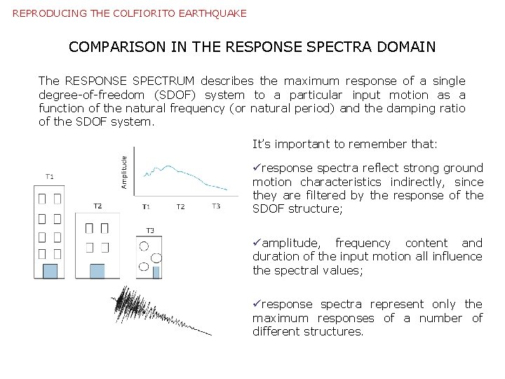
REPRODUCING THE COLFIORITO EARTHQUAKE COMPARISON IN THE RESPONSE SPECTRA DOMAIN The RESPONSE SPECTRUM describes the maximum response of a single degree-of-freedom (SDOF) system to a particular input motion as a function of the natural frequency (or natural period) and the damping ratio of the SDOF system. It’s important to remember that: üresponse spectra reflect strong ground motion characteristics indirectly, since they are filtered by the response of the SDOF structure; üamplitude, frequency content and duration of the input motion all influence the spectral values; üresponse spectra represent only the maximum responses of a number of different structures.

Larry

ALMA MATER STUDIORUM Dipartimento di Fisica dell’Università degli Studi di Bologna Dottorato in Geofisica, XVI ciclo PREDICTING THE GROUND MOTION: TWO DIFFERENT POINTS OF VIEW Laura Scognamiglio

OBJECTIVES The intention of this dissertation is to look into the empirical and semi-empirical approach for estimating strong ground motion. The two different methods were investigated for understanding their potentials for being used in the evaluation of the earthquake-induced ground motion: • Regression analyses on background seismicity • Strong ground motion evaluation with empirical Green’s function

EARTHQUAKE GROUND MOTION ESTIMATION TECNIQUES: 1. Theoretical evaluation 2. Semi-Empirical approach 3. Regression Techniques

Score for 100 models