Finding Dominators in Flowgraphs Loukas Georgiadis COS 423

Finding Dominators in Flowgraphs Loukas Georgiadis COS 423 - 03/29/2004 1

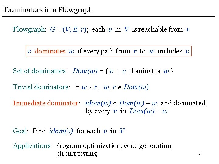
Dominators in a Flowgraph: G = (V, E, r); each v in V is reachable from r v dominates w if every path from r to w includes v Set of dominators: Dom(w) = { v | v dominates w } Trivial dominators: w r, w, r Dom(w) Immediate dominator: idom(w) Dom(w) – w and dominated by every v in Dom(w) – w Goal: Find idom(v) for each v in V Applications: Program optimization, code generation, circuit testing 2

Application: Loop Optimizations Loop optimizations typically make a program much more efficient since a large fraction of the total running time is spent on loops. Dominators can be used to detect loops. 3

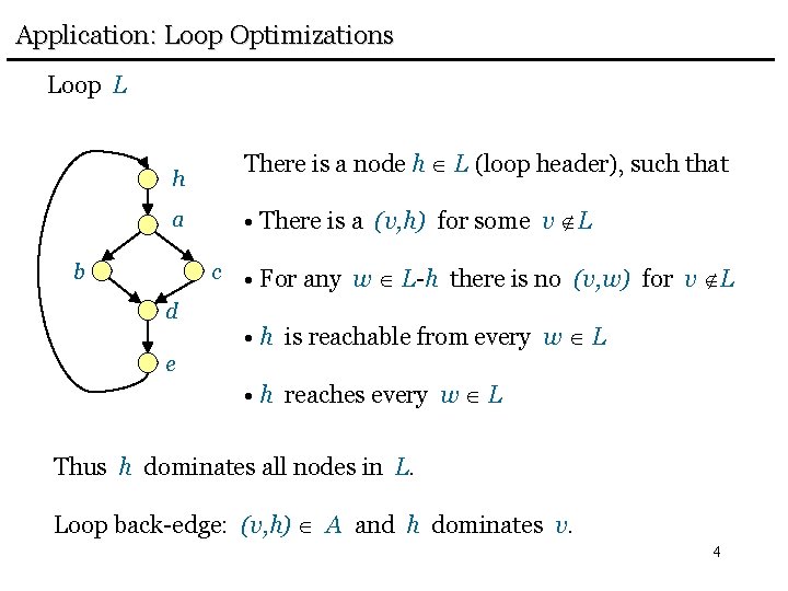
Application: Loop Optimizations Loop L There is a node h L (loop header), such that h • There is a (v, h) for some v L a b c d • For any w L-h there is no (v, w) for v L • h is reachable from every w L e • h reaches every w L Thus h dominates all nodes in L. Loop back-edge: (v, h) A and h dominates v. 4

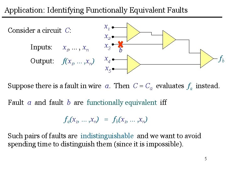
Application: Identifying Functionally Equivalent Faults Consider a circuit C: Inputs: x 1, … , x n Output: f(x 1, … , xn) x 1 x 2 x 3 b x 4 x 5 fb Suppose there is a fault in wire a. Then C = Ca evaluates fa instead. Fault a and fault b are functionally equivalent iff fa(x 1, … , xn) = fb(x 1, … , xn) Such pairs of faults are indistinguishable and we want to avoid spending time to distinguish them (since it is impossible). 5

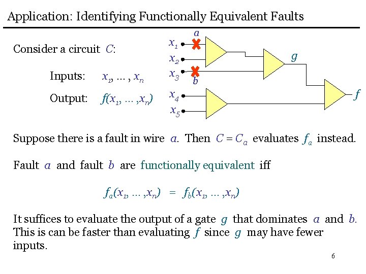
Application: Identifying Functionally Equivalent Faults Consider a circuit C: Inputs: x 1, … , x n Output: f(x 1, … , xn) x 1 x 2 x 3 a g b x 4 x 5 f Suppose there is a fault in wire a. Then C = Ca evaluates fa instead. Fault a and fault b are functionally equivalent iff fa(x 1, … , xn) = fb(x 1, … , xn) It suffices to evaluate the output of a gate g that dominates a and b. This is can be faster than evaluating f since g may have fewer inputs. 6

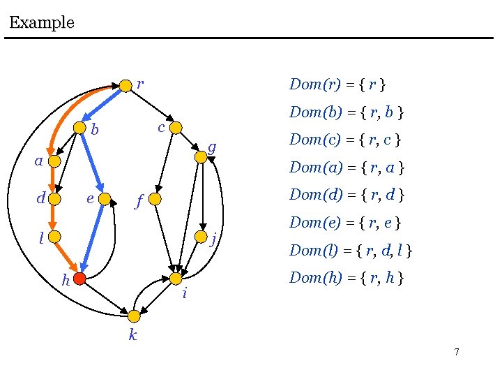
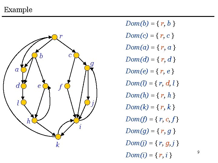
Example r Dom(r) = { r } Dom(b) = { r, b } c b g a Dom(c) = { r, c } Dom(a) = { r, a } d e Dom(d) = { r, d } f l j h i Dom(e) = { r, e } Dom(l) = { r, d, l } Dom(h) = { r, h } k 7

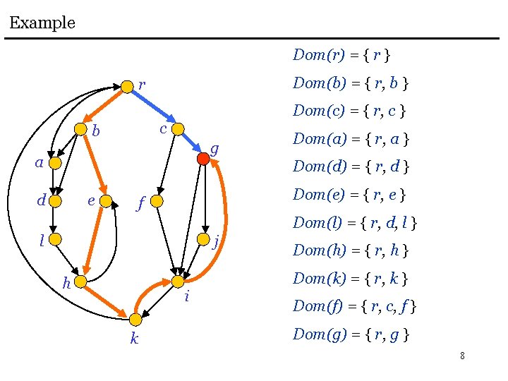
Example Dom(r) = { r } Dom(b) = { r, b } r Dom(c) = { r, c } c b g a Dom(a) = { r, a } Dom(d) = { r, d } d e Dom(e) = { r, e } f Dom(l) = { r, d, l } l j Dom(h) = { r, h } Dom(k) = { r, k } h i k Dom(f) = { r, c, f } Dom(g) = { r, g } 8

Example Dom(b) = { r, b } Dom(c) = { r, c } r Dom(a) = { r, a } c b g a Dom(d) = { r, d } Dom(e) = { r, e } d e Dom(l) = { r, d, l } f Dom(h) = { r, h } l j Dom(k) = { r, k } Dom(f) = { r, c, f } h i k Dom(g) = { r, g } Dom(j) = { r, g, j } Dom(i) = { r, i } 9

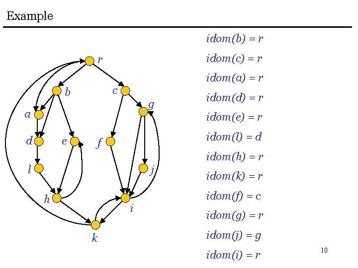
Example idom(b) = r idom(c) = r r idom(a) = r c b g a idom(d) = r idom(e) = r d e idom(l) = d f idom(h) = r l j idom(k) = r idom(f) = c h i k idom(g) = r idom(j) = g idom(i) = r 10

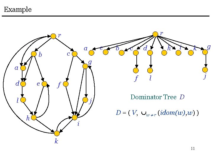
Example r r c b b c d h i g k g a d e a e f f l j j l Dominator Tree D D = ( V, w r (idom(w), w) ) h i k 11

A Straightforward Algorithm Purdom-Moore [1972]: for all v in V – r do remove v from G R(v) unreachable vertices for all u in R(v) do Dom(u) { v } done The running time is O(n m). Also very slow in practice. 12

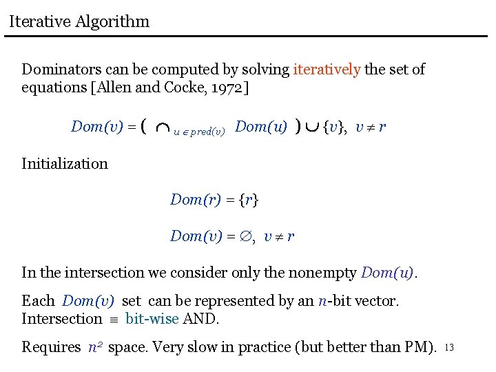
Iterative Algorithm Dominators can be computed by solving iteratively the set of equations [Allen and Cocke, 1972] Dom(v) = ( u pred(v) Dom(u) ) {v}, v r Initialization Dom(r) = {r} Dom(v) = , v r In the intersection we consider only the nonempty Dom(u). Each Dom(v) set can be represented by an n-bit vector. Intersection bit-wise AND. Requires n 2 space. Very slow in practice (but better than PM). 13

Iterative Algorithm Efficient implementation [Cooper, Harvey and Kennedy 2000] dfs(r) T {r} changed true while ( changed ) do changed false for all v in V – r in reverse postorder do x nca(pred(v)) if x parent(v) then parent(v) x changed true end done 14

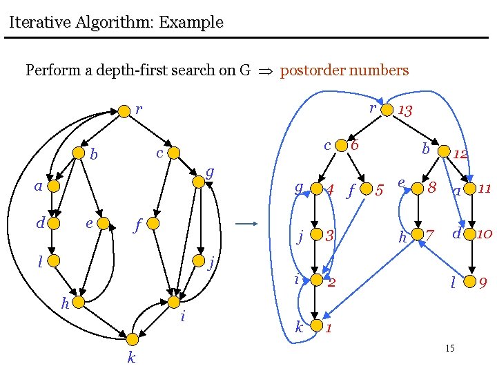
Iterative Algorithm: Example Perform a depth-first search on G postorder numbers r r c c b g a d e f l j h i k 13 6 g 4 f j 3 i 2 k 1 b 12 5 e 8 a 11 h 7 d 10 l 9 15

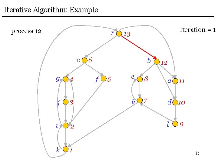
Iterative Algorithm: Example process 12 r c g 4 j 3 i 2 k 1 iteration = 1 13 6 b f 5 12 e 8 a 11 h 7 d 10 l 9 16

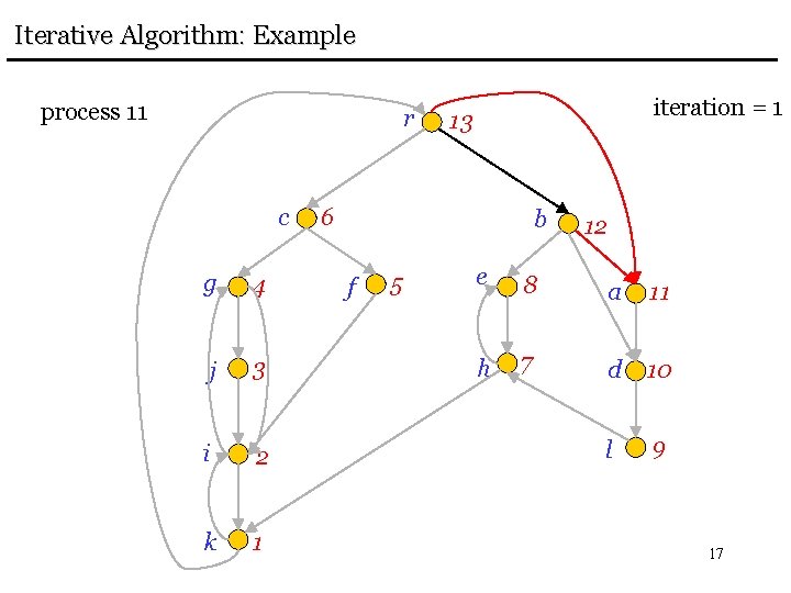
Iterative Algorithm: Example process 11 r c g 4 j 3 i 2 k 1 iteration = 1 13 6 b f 5 12 e 8 a 11 h 7 d 10 l 9 17

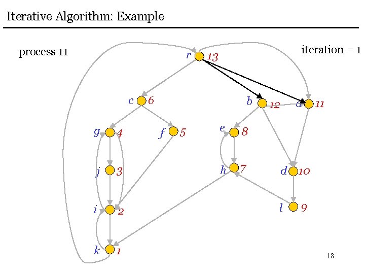
Iterative Algorithm: Example process 11 r c g 4 j 3 i 2 k 1 iteration = 1 13 6 b f 5 e 8 h 7 12 a d 10 l 9 11 18

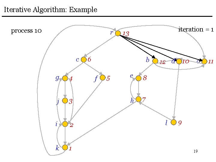
Iterative Algorithm: Example process 10 r c g 4 j 3 i 2 k 1 iteration = 1 13 6 b f 5 e 8 h 7 12 d l 10 a 9 19 11

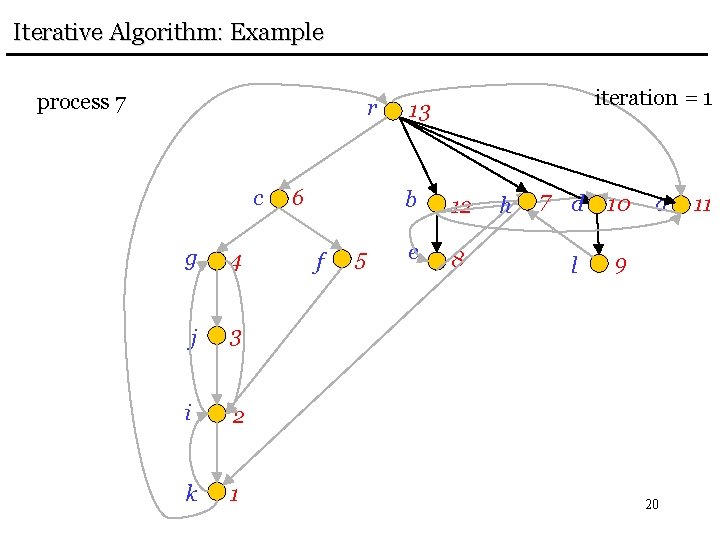
Iterative Algorithm: Example process 7 r c g 4 j 3 i 2 k 1 6 f 5 iteration = 1 13 b 12 e 8 h 7 d 10 l 9 a 20 11

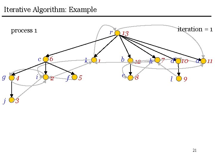
Iterative Algorithm: Example process 1 g 4 j 3 r c 6 i 2 k f 5 1 iteration = 1 13 b 12 e 8 h 7 d 10 l 9 a 21 11

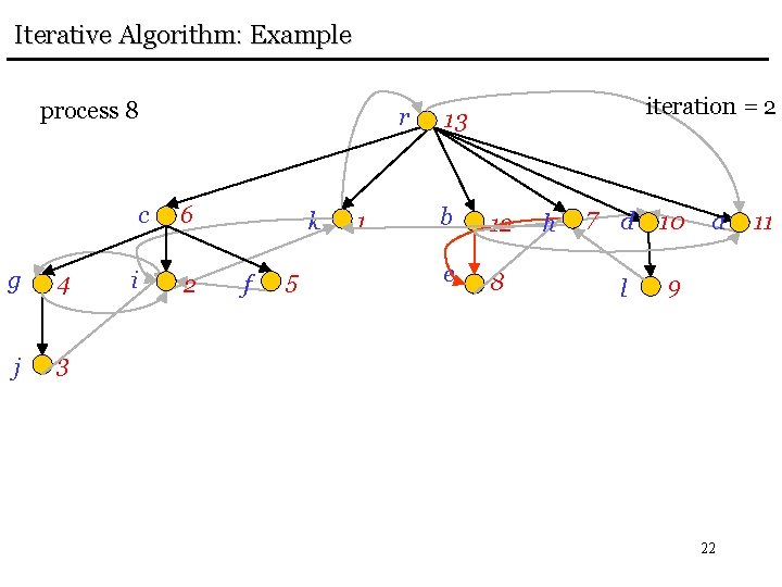
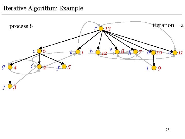
Iterative Algorithm: Example process 8 g 4 j 3 r c 6 i 2 k f 5 1 iteration = 2 13 b 12 e 8 h 7 d 10 l 9 a 22 11

Iterative Algorithm: Example process 8 g 4 j 3 r c 6 i 2 k f 5 1 b iteration = 2 13 12 e 8 h 7 d 10 l 9 a 23 11

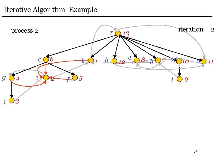
Iterative Algorithm: Example process 2 g 4 j 3 r c 6 i 2 k f 5 1 b iteration = 2 13 12 e 8 h 7 d 10 l 9 a 24 11

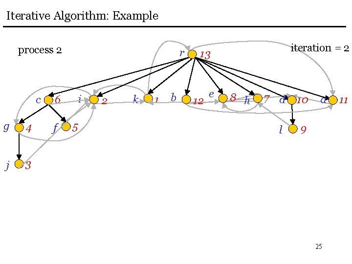
Iterative Algorithm: Example process 2 c g 4 j 3 r i 6 f 5 2 k 1 b iteration = 2 13 12 e 8 h 7 d 10 l 9 a 25 11

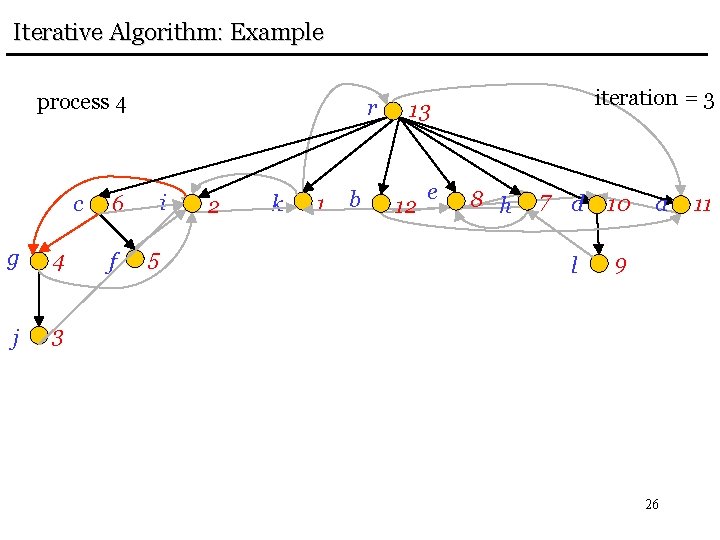
Iterative Algorithm: Example process 4 c g 4 j 3 r i 6 f 5 2 k 1 b iteration = 3 13 12 e 8 h 7 d 10 l 9 a 26 11

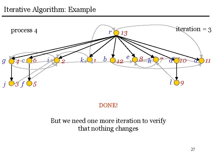
Iterative Algorithm: Example process 4 g 4 c 6 j 3 f 5 r i 2 k 1 b iteration = 3 13 12 e 8 h 7 d l 10 a 9 DONE! But we need one more iteration to verify that nothing changes 27 11

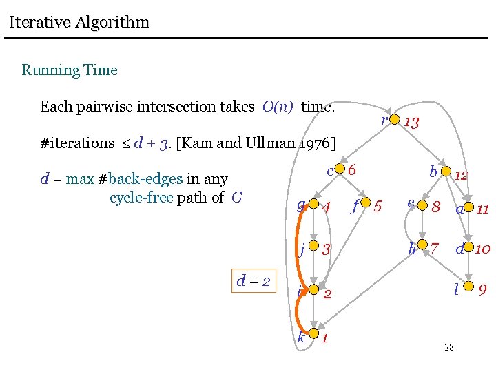
Iterative Algorithm Running Time Each pairwise intersection takes O(n) time. r 13 #iterations d + 3. [Kam and Ullman 1976] d = max #back-edges in any cycle-free path of G d=2 c 6 g 4 j 3 i 2 k 1 f 5 b 12 8 a 11 h 7 d 10 e l 28 9

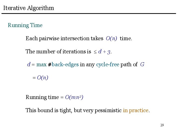
Iterative Algorithm Running Time Each pairwise intersection takes O(n) time. The number of iterations is d + 3. d = max #back-edges in any cycle-free path of G = O(n) Running time = O(mn 2) This bound is tight, but very pessimistic in practice. 29

A Fast Dominator Algorithm Lengauer-Tarjan [1979]: O(n (m, n)) time A simpler version runs in O(m log 2+ m/n n) time 30

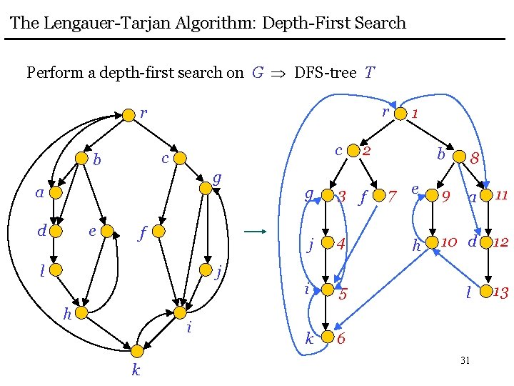
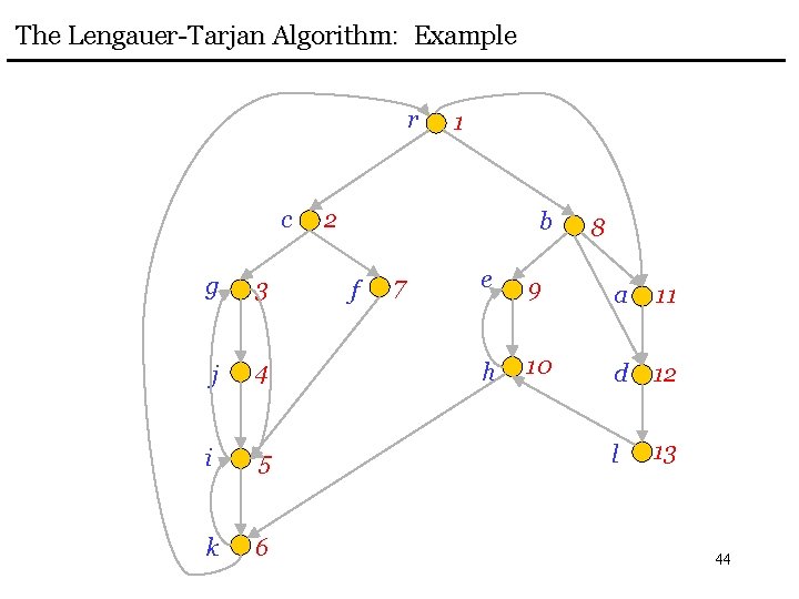
The Lengauer-Tarjan Algorithm: Depth-First Search Perform a depth-first search on G DFS-tree T r r c c b g a d e f l j h i k 1 2 g 3 f j 4 i 5 k 6 b 7 e h 9 8 a 11 10 d 12 l 31 13

The Lengauer-Tarjan Algorithm: Depth-First Search Tree T : We refer to the vertices by their DFS numbers: v < w : v was visited by DFS before w Notation v * w : v is an ancestor of w in T v + w : v is a proper ancestor of w in T parent(v) : parent of v in T Property 1 v, w such that v w, (v, w) E v * w 32

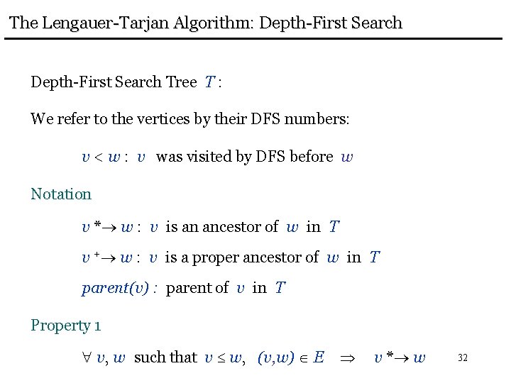
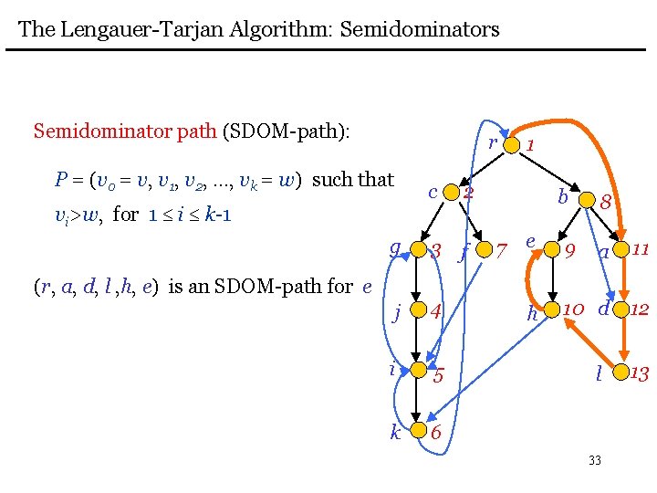
The Lengauer-Tarjan Algorithm: Semidominators Semidominator path (SDOM-path): r P = (v 0 = v, v 1, v 2, …, vk = w) such that c vi>w, for 1 i k-1 2 g 3 f j 4 i 5 k 6 (r, a, d, l , h, e) is an SDOM-path for e 1 b 7 e h 9 8 a 11 10 d 12 l 33 13

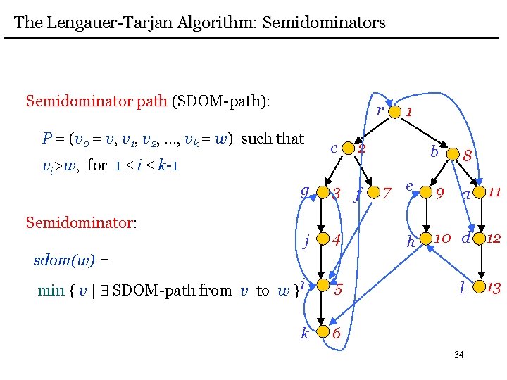
The Lengauer-Tarjan Algorithm: Semidominators Semidominator path (SDOM-path): r P = (v 0 = v, v 1, v 2, …, vk = w) such that c vi>w, for 1 i k-1 2 g 3 f j 4 min { v | SDOM-path from v to w }i 5 k 6 Semidominator: 1 b 7 e h 9 8 a 11 10 d 12 sdom(w) = l 34 13

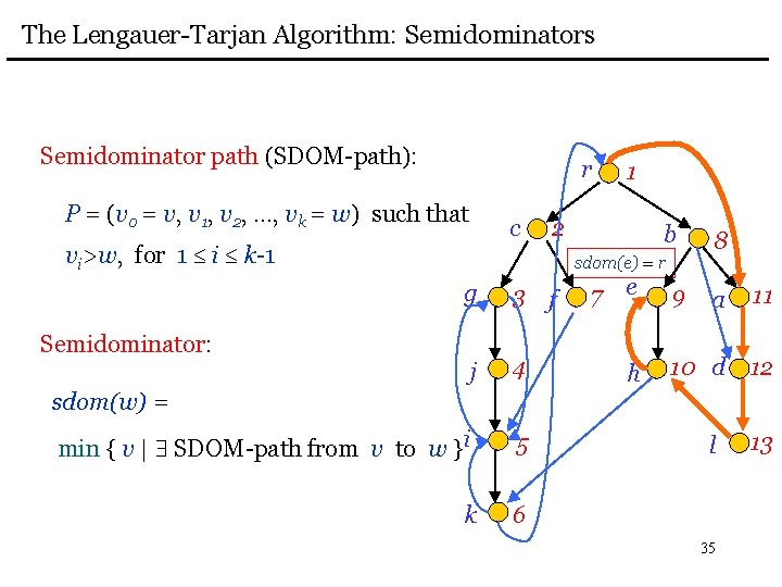
The Lengauer-Tarjan Algorithm: Semidominators Semidominator path (SDOM-path): r P = (v 0 = v, v 1, v 2, …, vk = w) such that c vi>w, for 1 i k-1 1 2 b sdom(e) = r g 3 f j 4 min { v | SDOM-path from v to w }i 5 k 6 Semidominator: 7 e h 9 8 a 11 10 d 12 sdom(w) = l 35 13

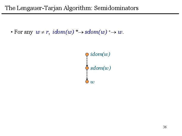
The Lengauer-Tarjan Algorithm: Semidominators • For any w r, idom(w) * sdom(w) + w. idom(w) sdom(w) w 36

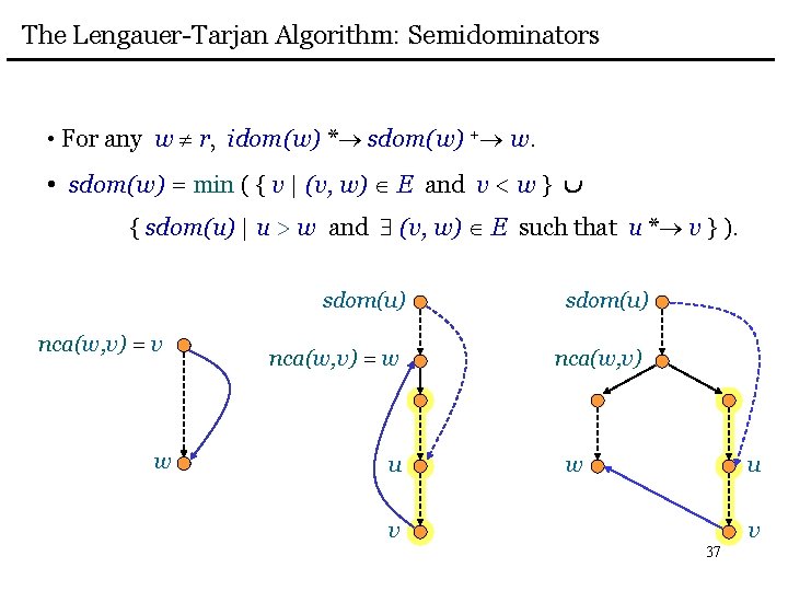
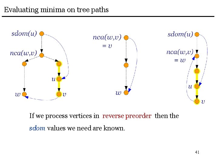
The Lengauer-Tarjan Algorithm: Semidominators • For any w r, idom(w) * sdom(w) + w. • sdom(w) = min ( { v | (v, w) E and v < w } { sdom(u) | u > w and (v, w) E such that u * v } ). nca(w, v) = v w sdom(u) nca(w, v) = w nca(w, v) u w u v v 37

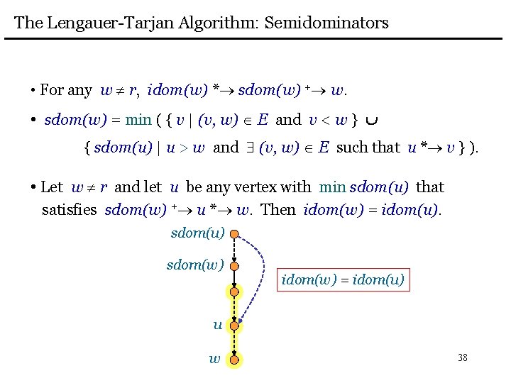
The Lengauer-Tarjan Algorithm: Semidominators • For any w r, idom(w) * sdom(w) + w. • sdom(w) = min ( { v | (v, w) E and v < w } { sdom(u) | u > w and (v, w) E such that u * v } ). • Let w r and let u be any vertex with min sdom(u) that satisfies sdom(w) + u * w. Then idom(w) = idom(u). sdom(u) sdom(w) idom(w) = idom(u) u w 38

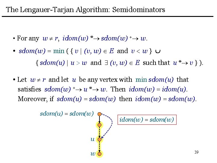
The Lengauer-Tarjan Algorithm: Semidominators • For any w r, idom(w) * sdom(w) + w. • sdom(w) = min ( { v | (v, w) E and v < w } { sdom(u) | u > w and (v, w) E such that u * v } ). • Let w r and let u be any vertex with min sdom(u) that satisfies sdom(w) + u * w. Then idom(w) = idom(u). Moreover, if sdom(u) = sdom(w) then idom(w) = sdom(w). sdom(u) = sdom(w) idom(w) = sdom(w) u w 39

The Lengauer-Tarjan Algorithm Overview of the Algorithm 1. Carry out a DFS. 2. Process the vertices in reverse preorder. For vertex w, compute sdom(w). 3. Implicitly define idom(w). 4. Explicitly define idom(w) by a preorder pass. 40

Evaluating minima on tree paths If we process vertices in reverse preorder then the sdom values we need are known. 41

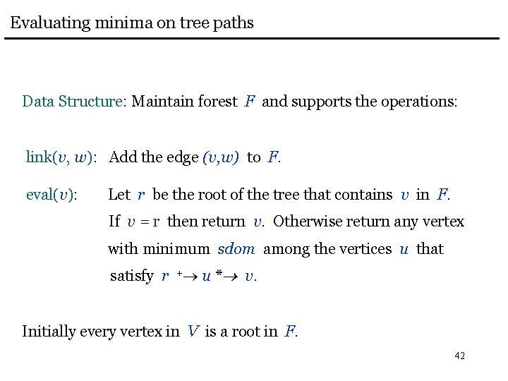
Evaluating minima on tree paths Data Structure: Maintain forest F and supports the operations: link(v, w): Add the edge (v, w) to F. eval(v): Let r be the root of the tree that contains v in F. If v = r then return v. Otherwise return any vertex with minimum sdom among the vertices u that satisfy r + u * v. Initially every vertex in V is a root in F. 42

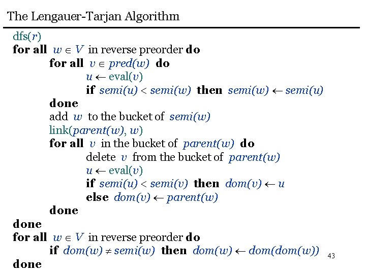
The Lengauer-Tarjan Algorithm dfs(r) for all w V in reverse preorder do for all v pred(w) do u eval(v) if semi(u) < semi(w) then semi(w) semi(u) done add w to the bucket of semi(w) link(parent(w), w) for all v in the bucket of parent(w) do delete v from the bucket of parent(w) u eval(v) if semi(u) < semi(v) then dom(v) u else dom(v) parent(w) done for all w V in reverse preorder do if dom(w) semi(w) then dom(w)) done 43

The Lengauer-Tarjan Algorithm: Example r c g 3 j 4 i 5 k 6 1 2 b f 7 8 e 9 a 11 h 10 d 12 l 13 44

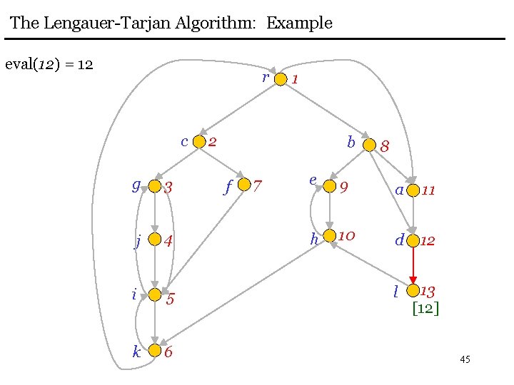
The Lengauer-Tarjan Algorithm: Example eval(12) = 12 r c g 3 j 4 i 5 k 6 1 2 b f 7 8 e 9 a 11 h 10 d 12 l 13 [12] 45

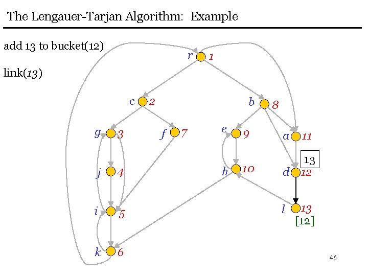
The Lengauer-Tarjan Algorithm: Example add 13 to bucket(12) r 1 link(13) c g 3 j 4 i 5 k 6 2 b f 7 e h 9 10 8 a 11 d 13 12 l 13 [12] 46

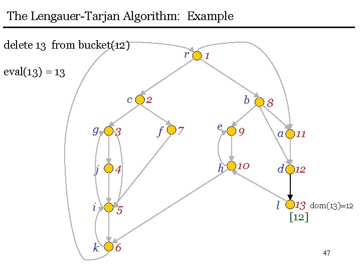
The Lengauer-Tarjan Algorithm: Example delete 13 from bucket(12) r 1 eval(13) = 13 c g 3 j 4 i 5 k 6 2 b f 7 8 e 9 a 11 h 10 d 12 l 13 dom(13)=12 [12] 47

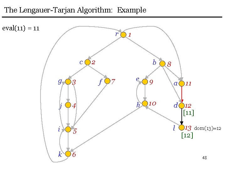
The Lengauer-Tarjan Algorithm: Example eval(11) = 11 r c g 3 j 4 i 5 k 6 1 2 b f 7 8 e 9 a 11 h 10 d 12 [11] l 13 dom(13)=12 [12] 48

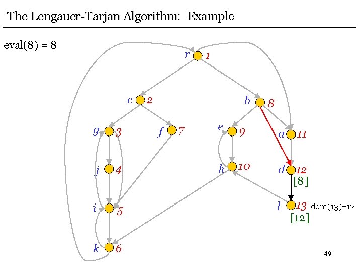
The Lengauer-Tarjan Algorithm: Example eval(8) = 8 r c g 3 j 4 i 5 k 6 1 2 b f 7 8 e 9 a 11 h 10 d 12 [8] l 13 dom(13)=12 [12] 49

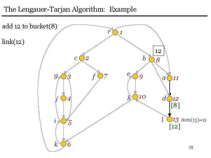
The Lengauer-Tarjan Algorithm: Example add 12 to bucket(8) r 1 link(12) c g 3 j 4 i 5 k 6 2 b f 7 12 8 e 9 a 11 h 10 d 12 [8] l 13 dom(13)=12 [12] 50

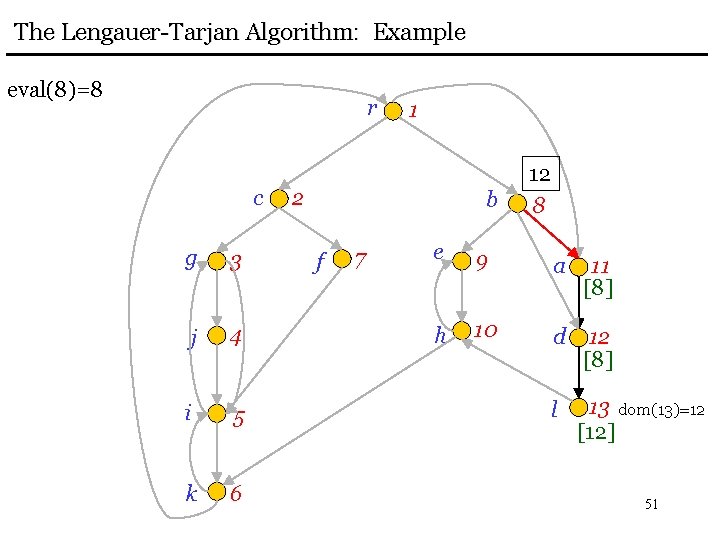
The Lengauer-Tarjan Algorithm: Example eval(8)=8 r c g 3 j 4 i 5 k 6 1 2 b f 7 12 8 e 9 a 11 [8] h 10 d 12 [8] l 13 dom(13)=12 [12] 51

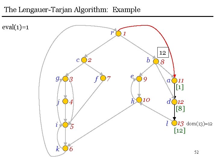
The Lengauer-Tarjan Algorithm: Example eval(1)=1 r c g 3 j 4 i 5 k 6 1 2 b f 7 12 8 e 9 a 11 [1] h 10 d 12 [8] l 13 dom(13)=12 [12] 52

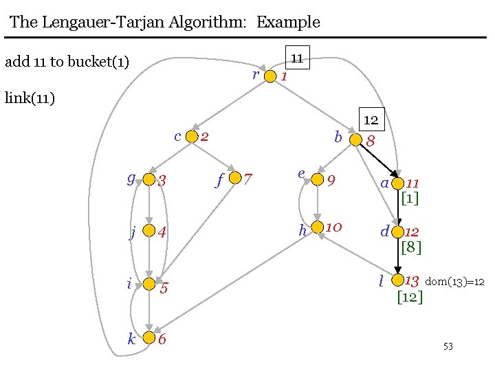
The Lengauer-Tarjan Algorithm: Example add 11 to bucket(1) r 11 1 link(11) c g 3 j 4 i 5 k 6 2 b f 7 12 8 e 9 a 11 [1] h 10 d 12 [8] l 13 dom(13)=12 [12] 53

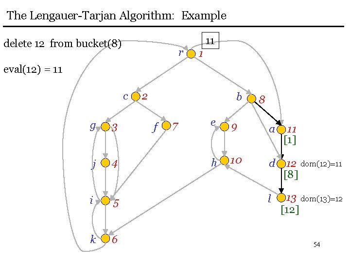
The Lengauer-Tarjan Algorithm: Example delete 12 from bucket(8) r 11 1 eval(12) = 11 c g 3 j 4 i 5 k 6 2 b f 7 8 e 9 a 11 [1] h 10 d 12 dom(12)=11 [8] l 13 dom(13)=12 [12] 54

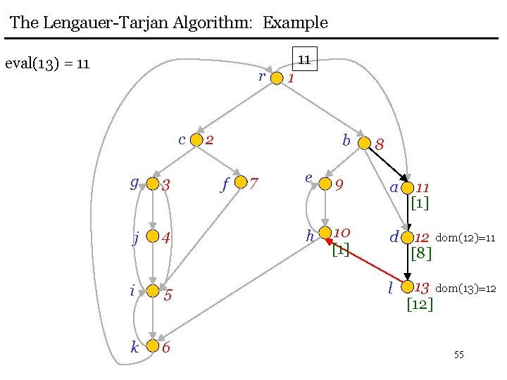
The Lengauer-Tarjan Algorithm: Example eval(13) = 11 r c g 3 j 4 i 5 k 6 11 1 2 b f 7 8 e 9 a 11 [1] h 10 [1] d 12 dom(12)=11 [8] l 13 dom(13)=12 [12] 55

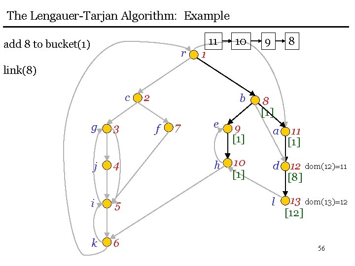
The Lengauer-Tarjan Algorithm: Example add 8 to bucket(1) r 11 10 9 8 b 8 [1] 1 link(8) c g 3 j 4 i 5 k 6 2 f 7 e 9 [1] a 11 [1] h 10 [1] d 12 dom(12)=11 [8] l 13 dom(13)=12 [12] 56

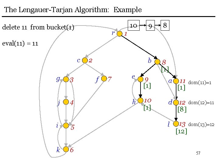
The Lengauer-Tarjan Algorithm: Example delete 11 from bucket(1) r 10 9 8 b 8 [1] 1 eval(11) = 11 c g 3 j 4 i 5 k 6 2 f 7 e 9 [1] a 11 [1] h 10 [1] d 12 dom(12)=11 [8] l 13 dom(13)=12 [12] dom(11)=1 57

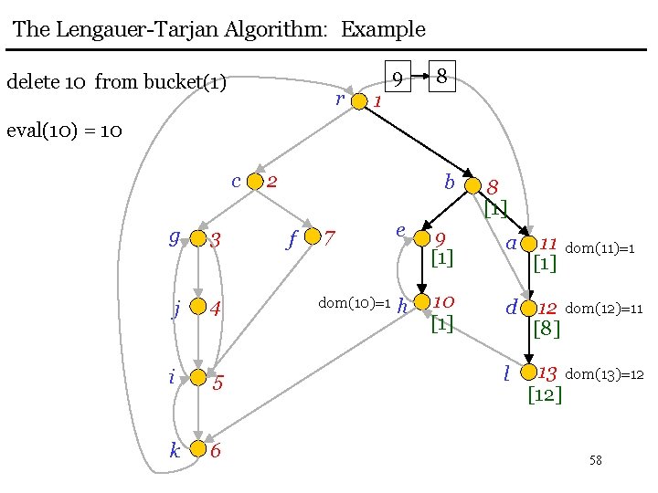
The Lengauer-Tarjan Algorithm: Example delete 10 from bucket(1) r 9 8 1 eval(10) = 10 c g 3 j 4 i 5 k 6 2 b f 7 dom(10)=1 8 [1] e 9 [1] a 11 [1] h 10 [1] d 12 dom(12)=11 [8] l 13 dom(13)=12 [12] dom(11)=1 58

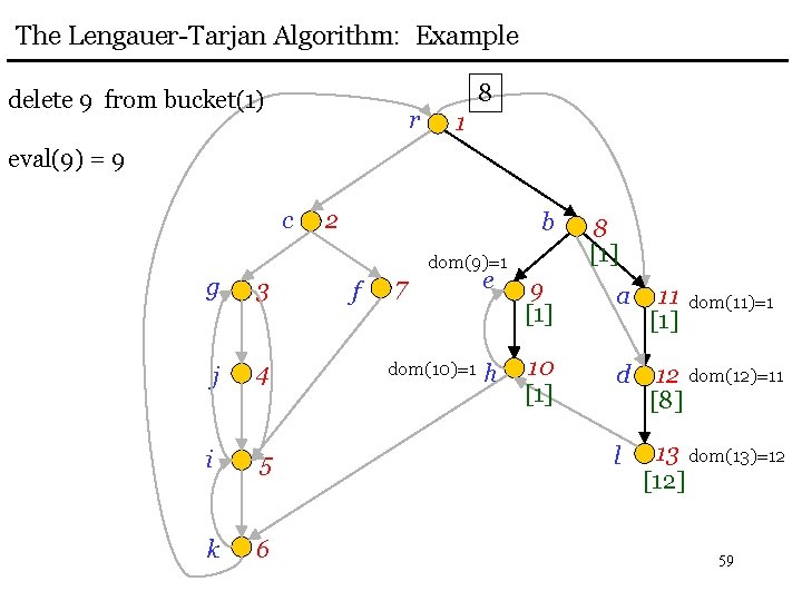
The Lengauer-Tarjan Algorithm: Example delete 9 from bucket(1) r 8 1 eval(9) = 9 c 2 b dom(9)=1 g 3 j 4 i 5 k 6 f 7 dom(10)=1 8 [1] e 9 [1] a 11 [1] h 10 [1] d 12 dom(12)=11 [8] l 13 dom(13)=12 [12] dom(11)=1 59

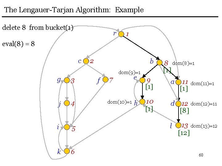
The Lengauer-Tarjan Algorithm: Example delete 8 from bucket(1) r 1 eval(8) = 8 c 2 b dom(9)=1 g 3 j 4 i 5 k 6 f 7 dom(10)=1 8 dom(8)=1 [1] e 9 [1] a 11 [1] h 10 [1] d 12 dom(12)=11 [8] l 13 dom(13)=12 [12] dom(11)=1 60

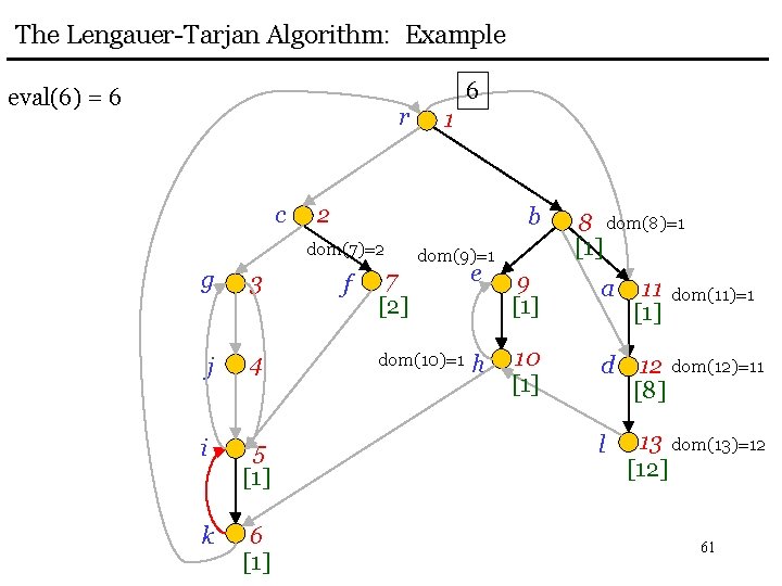
The Lengauer-Tarjan Algorithm: Example eval(6) = 6 r c 3 j 4 i 5 [1] k 6 [1] 1 2 b dom(7)=2 g 6 f dom(9)=1 8 dom(8)=1 [1] 7 [2] e 9 [1] a 11 [1] dom(10)=1 h 10 [1] d 12 dom(12)=11 [8] l 13 dom(13)=12 [12] dom(11)=1 61

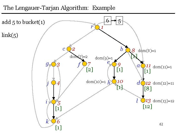
The Lengauer-Tarjan Algorithm: Example add 5 to bucket(1) r 6 5 1 link(5) c 2 b dom(7)=2 g 3 j 4 i 5 [1] k 6 [1] f dom(9)=1 8 dom(8)=1 [1] 7 [2] e 9 [1] a 11 [1] dom(10)=1 h 10 [1] d 12 dom(12)=11 [8] l 13 dom(13)=12 [12] dom(11)=1 62

The Lengauer-Tarjan Algorithm: Example eval(3) = 3 r c 3 j 4 [3] i 5 [1] k 6 [1] 5 1 2 b dom(7)=2 g 6 f dom(9)=1 8 dom(8)=1 [1] 7 [2] e 9 [1] a 11 [1] dom(10)=1 h 10 [1] d 12 dom(12)=11 [8] l 13 dom(13)=12 [12] dom(11)=1 63

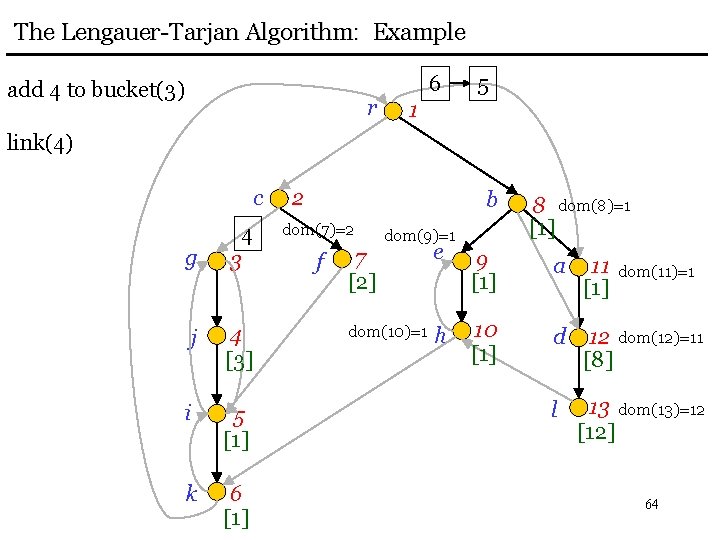
The Lengauer-Tarjan Algorithm: Example add 4 to bucket(3) r 6 5 1 link(4) c g 4 3 j 4 [3] i 5 [1] k 6 [1] 2 b dom(7)=2 f dom(9)=1 8 dom(8)=1 [1] 7 [2] e 9 [1] a 11 [1] dom(10)=1 h 10 [1] d 12 dom(12)=11 [8] l 13 dom(13)=12 [12] dom(11)=1 64

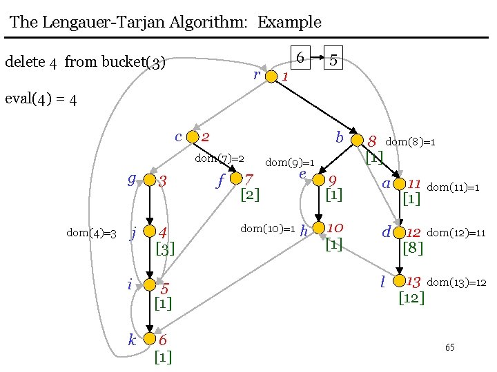
The Lengauer-Tarjan Algorithm: Example delete 4 from bucket(3) r 6 5 1 eval(4) = 4 c 2 b dom(7)=2 dom(4)=3 g 3 j 4 [3] i 5 [1] k 6 [1] f dom(9)=1 8 dom(8)=1 [1] 7 [2] e 9 [1] a 11 [1] dom(10)=1 h 10 [1] d 12 dom(12)=11 [8] l 13 dom(13)=12 [12] dom(11)=1 65

The Lengauer-Tarjan Algorithm: Example eval(2) = 2 r c dom(4)=3 3 [2] j 4 [3] i 5 [1] k 6 [1] 5 1 2 b dom(7)=2 g 6 f dom(9)=1 8 dom(8)=1 [1] 7 [2] e 9 [1] a 11 [1] dom(10)=1 h 10 [1] d 12 dom(12)=11 [8] l 13 dom(13)=12 [12] dom(11)=1 66

The Lengauer-Tarjan Algorithm: Example eval(5) = 5 r c dom(4)=3 3 [1] j 4 [3] i 5 [1] k 6 [1] 5 1 2 b dom(7)=2 g 6 f dom(9)=1 8 dom(8)=1 [1] 7 [2] e 9 [1] a 11 [1] dom(10)=1 h 10 [1] d 12 dom(12)=11 [8] l 13 dom(13)=12 [12] dom(11)=1 67

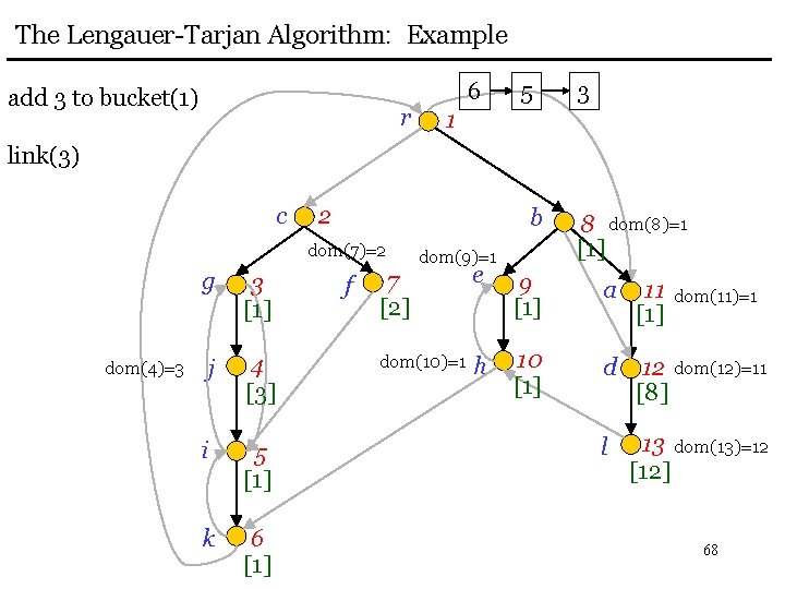
The Lengauer-Tarjan Algorithm: Example add 3 to bucket(1) r 6 5 3 1 link(3) c 2 b dom(7)=2 dom(4)=3 g 3 [1] j 4 [3] i 5 [1] k 6 [1] f dom(9)=1 8 dom(8)=1 [1] 7 [2] e 9 [1] a 11 [1] dom(10)=1 h 10 [1] d 12 dom(12)=11 [8] l 13 dom(13)=12 [12] dom(11)=1 68

The Lengauer-Tarjan Algorithm: Example eval(1) = 1 r c dom(4)=3 3 [1] j 4 [3] i 5 [1] k 6 [1] f 5 3 1 2 [1] b dom(7)=2 g 6 dom(9)=1 8 dom(8)=1 [1] 7 [2] e 9 [1] a 11 [1] dom(10)=1 h 10 [1] d 12 dom(12)=11 [8] l 13 dom(13)=12 [12] dom(11)=1 69

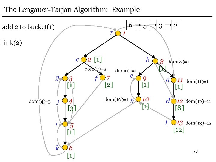
The Lengauer-Tarjan Algorithm: Example add 2 to bucket(1) r 6 5 3 2 1 link(2) c 2 [1] b dom(7)=2 dom(4)=3 g 3 [1] j 4 [3] i 5 [1] k 6 [1] f dom(9)=1 8 dom(8)=1 [1] 7 [2] e 9 [1] a 11 [1] dom(10)=1 h 10 [1] d 12 dom(12)=11 [8] l 13 dom(13)=12 [12] dom(11)=1 70

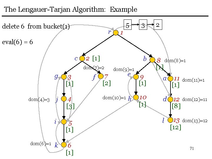
The Lengauer-Tarjan Algorithm: Example delete 6 from bucket(1) r 5 3 2 b 8 dom(8)=1 [1] 1 eval(6) = 6 c 2 [1] dom(7)=2 dom(4)=3 dom(6)=1 g 3 [1] j 4 [3] i 5 [1] k 6 [1] f dom(9)=1 7 [2] e 9 [1] a 11 [1] dom(10)=1 h 10 [1] d 12 dom(12)=11 [8] l 13 dom(13)=12 [12] dom(11)=1 71

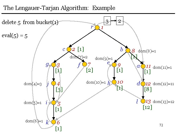
The Lengauer-Tarjan Algorithm: Example delete 5 from bucket(1) r 3 2 1 eval(5) = 5 c 2 [1] b dom(7)=2 dom(4)=3 dom(5)=1 dom(6)=1 g 3 [1] j 4 [3] i 5 [1] k 6 [1] f dom(9)=1 8 dom(8)=1 [1] 7 [2] e 9 [1] a 11 [1] dom(10)=1 h 10 [1] d 12 dom(12)=11 [8] l 13 dom(13)=12 [12] dom(11)=1 72

The Lengauer-Tarjan Algorithm: Example delete 3 from bucket(1) r 2 1 eval(3) = 3 c 2 [1] b dom(7)=2 dom(3)=1 g 3 [1] dom(4)=3 j 4 [3] i 5 [1] k 6 [1] dom(5)=1 dom(6)=1 f dom(9)=1 8 dom(8)=1 [1] 7 [2] e 9 [1] a 11 [1] dom(10)=1 h 10 [1] d 12 dom(12)=11 [8] l 13 dom(13)=12 [12] dom(11)=1 73

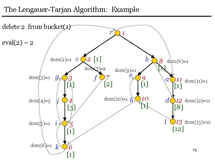
The Lengauer-Tarjan Algorithm: Example delete 2 from bucket(1) r 1 eval(2) = 2 dom(2)=1 c 2 [1] b dom(7)=2 dom(3)=1 g 3 [1] dom(4)=3 j 4 [3] i 5 [1] k 6 [1] dom(5)=1 dom(6)=1 f dom(9)=1 8 dom(8)=1 [1] 7 [2] e 9 [1] a 11 [1] dom(10)=1 h 10 [1] d 12 dom(12)=11 [8] l 13 dom(13)=12 [12] dom(11)=1 74

The Lengauer-Tarjan Algorithm: Example dom(12) semi(12) r 1 set dom(12)=dom(11) dom(2)=1 c 2 [1] b dom(7)=2 dom(3)=1 g 3 [1] dom(4)=3 j 4 [3] i 5 [1] k 6 [1] dom(5)=1 dom(6)=1 f dom(9)=1 8 dom(8)=1 [1] 7 [2] e 9 [1] a 11 [1] dom(10)=1 h 10 [1] d 12 dom(12)=1 [8] l 13 dom(13)=12 [12] dom(11)=1 75

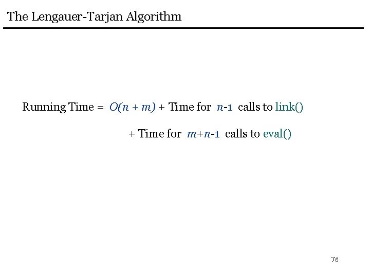
The Lengauer-Tarjan Algorithm Running Time = O(n + m) + Time for n-1 calls to link() + Time for m+n-1 calls to eval() 76

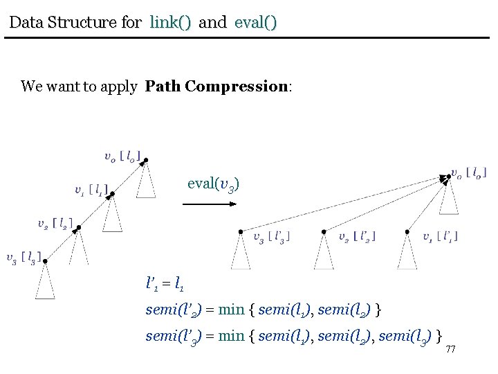
Data Structure for link() and eval() We want to apply Path Compression: eval(v 3) l’ 1 = l 1 semi(l’ 2) = min { semi(l 1), semi(l 2) } semi(l’ 3) = min { semi(l 1), semi(l 2), semi(l 3) } 77

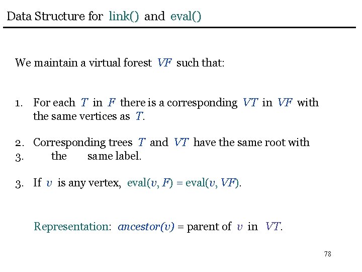
Data Structure for link() and eval() We maintain a virtual forest VF such that: 1. For each T in F there is a corresponding VT in VF with the same vertices as T. 2. Corresponding trees T and VT have the same root with 3. the same label. 3. If v is any vertex, eval(v, F) = eval(v, VF). Representation: ancestor(v) = parent of v in VT. 78

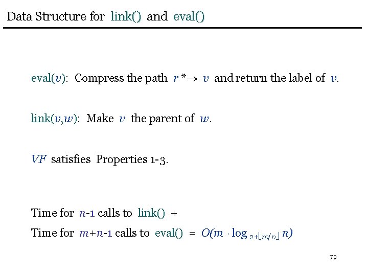
Data Structure for link() and eval() eval(v): Compress the path r * v and return the label of v. link(v, w): Make v the parent of w. VF satisfies Properties 1 -3. Time for n-1 calls to link() + Time for m+n-1 calls to eval() = O(m log 2+ m/n n) 79

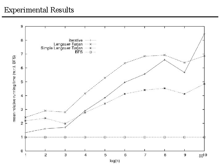
Experimental Results 80

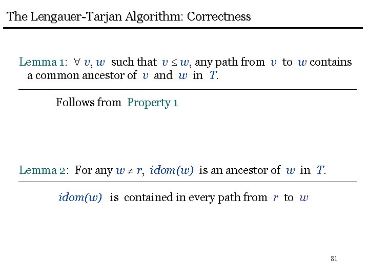
The Lengauer-Tarjan Algorithm: Correctness Lemma 1: v, w such that v w, any path from v to w contains a common ancestor of v and w in T. Follows from Property 1 Lemma 2: For any w r, idom(w) is an ancestor of w in T. idom(w) is contained in every path from r to w 81

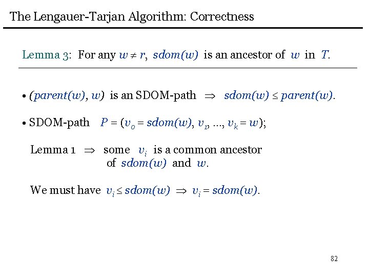
The Lengauer-Tarjan Algorithm: Correctness Lemma 3: For any w r, sdom(w) is an ancestor of w in T. • (parent(w), w) is an SDOM-path sdom(w) parent(w). • SDOM-path P = (v 0 = sdom(w), v 1, …, vk = w); Lemma 1 some vi is a common ancestor of sdom(w) and w. We must have vi sdom(w) vi = sdom(w). 82

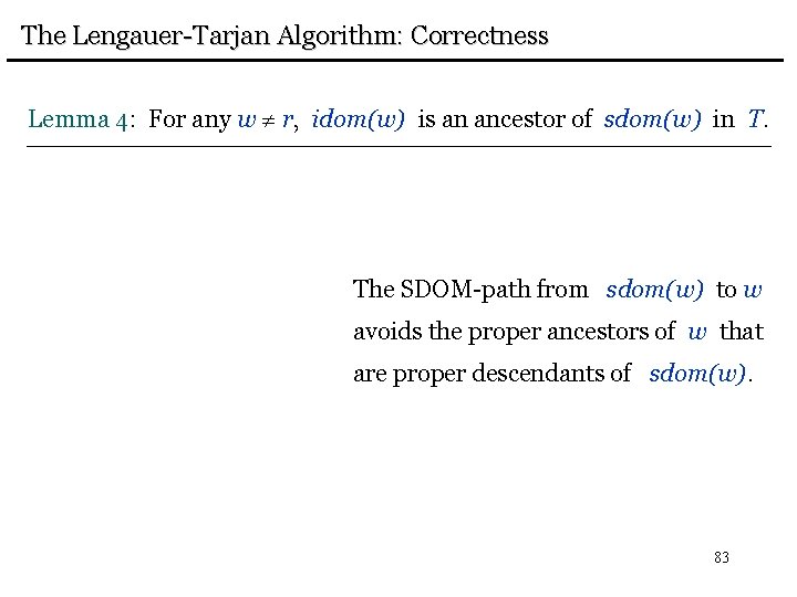
The Lengauer-Tarjan Algorithm: Correctness Lemma 4: For any w r, idom(w) is an ancestor of sdom(w) in T. The SDOM-path from sdom(w) to w avoids the proper ancestors of w that are proper descendants of sdom(w). 83

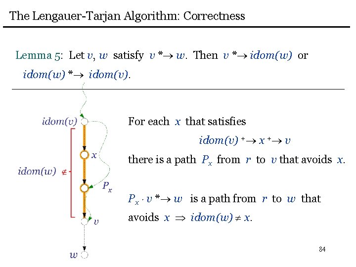
The Lengauer-Tarjan Algorithm: Correctness Lemma 5: Let v, w satisfy v * w. Then v * idom(w) or idom(w) * idom(v). For each x that satisfies idom(v) + x + v there is a path Px from r to v that avoids x. Px v * w is a path from r to w that avoids x idom(w) x. 84

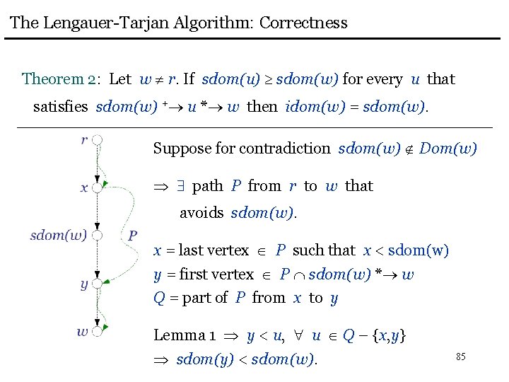
The Lengauer-Tarjan Algorithm: Correctness Theorem 2: Let w r. If sdom(u) sdom(w) for every u that satisfies sdom(w) + u * w then idom(w) = sdom(w). Suppose for contradiction sdom(w) Dom(w) path P from r to w that avoids sdom(w). x = last vertex P such that x < sdom(w) y = first vertex P sdom(w) * w Q = part of P from x to y Lemma 1 y < u, u Q – {x, y} sdom(y) < sdom(w). 85

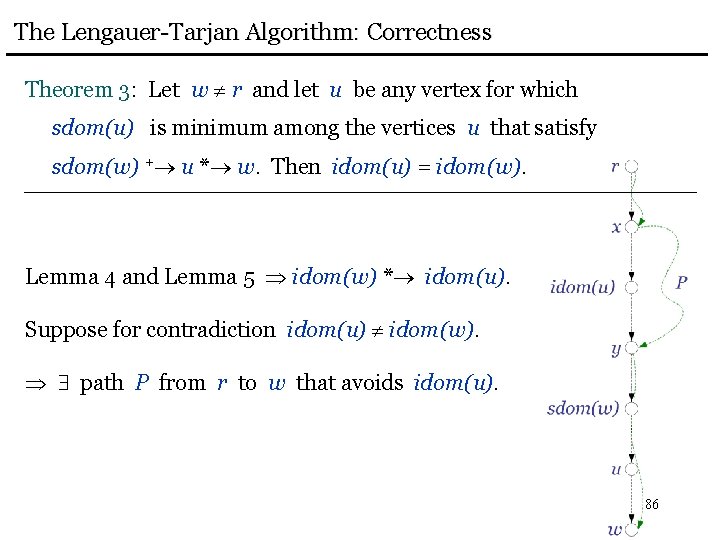
The Lengauer-Tarjan Algorithm: Correctness Theorem 3: Let w r and let u be any vertex for which sdom(u) is minimum among the vertices u that satisfy sdom(w) + u * w. Then idom(u) = idom(w). Lemma 4 and Lemma 5 idom(w) * idom(u). Suppose for contradiction idom(u) idom(w). path P from r to w that avoids idom(u). 86

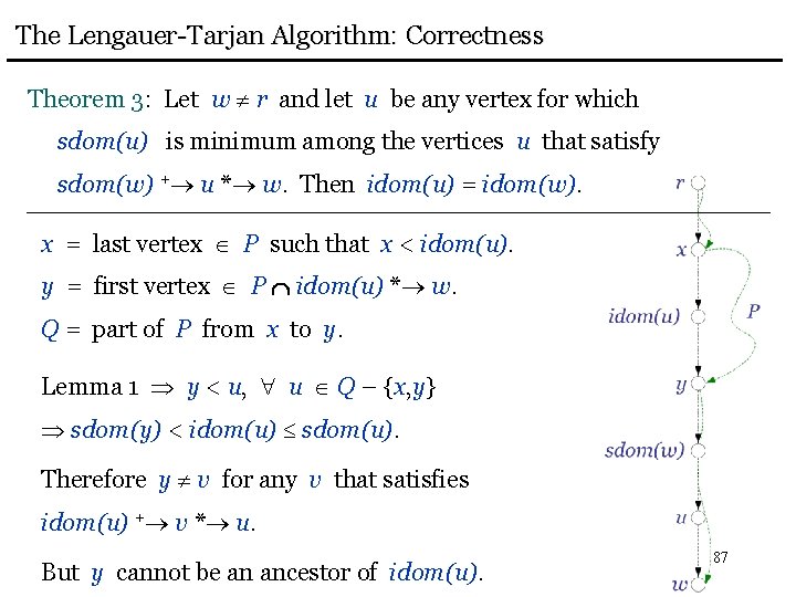
The Lengauer-Tarjan Algorithm: Correctness Theorem 3: Let w r and let u be any vertex for which sdom(u) is minimum among the vertices u that satisfy sdom(w) + u * w. Then idom(u) = idom(w). x = last vertex P such that x < idom(u). y = first vertex P idom(u) * w. Q = part of P from x to y. Lemma 1 y < u, u Q – {x, y} sdom(y) < idom(u) sdom(u). Therefore y v for any v that satisfies idom(u) + v * u. But y cannot be an ancestor of idom(u). 87

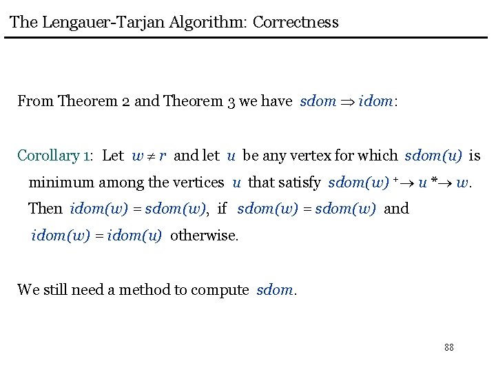
The Lengauer-Tarjan Algorithm: Correctness From Theorem 2 and Theorem 3 we have sdom idom: Corollary 1: Let w r and let u be any vertex for which sdom(u) is minimum among the vertices u that satisfy sdom(w) + u * w. Then idom(w) = sdom(w), if sdom(w) = sdom(w) and idom(w) = idom(u) otherwise. We still need a method to compute sdom. 88

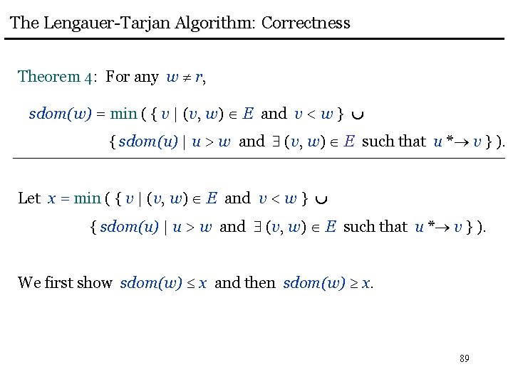
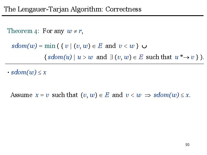
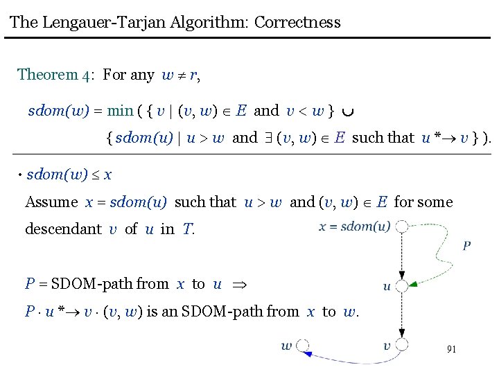
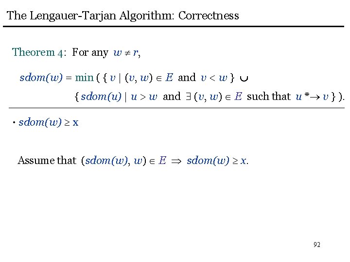
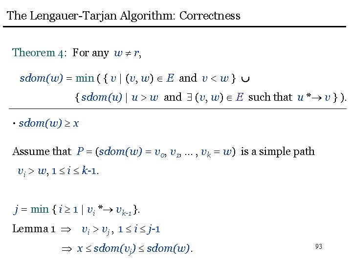
The Lengauer-Tarjan Algorithm: Correctness Theorem 4: For any w r, sdom(w) = min ( { v | (v, w) E and v < w } { sdom(u) | u > w and (v, w) E such that u * v } ). Let x = min ( { v | (v, w) E and v < w } { sdom(u) | u > w and (v, w) E such that u * v } ). We first show sdom(w) x and then sdom(w) x. 89

The Lengauer-Tarjan Algorithm: Correctness Theorem 4: For any w r, sdom(w) = min ( { v | (v, w) E and v < w } { sdom(u) | u > w and (v, w) E such that u * v } ). • sdom(w) x Assume x = v such that (v, w) E and v < w sdom(w) x. 90

The Lengauer-Tarjan Algorithm: Correctness Theorem 4: For any w r, sdom(w) = min ( { v | (v, w) E and v < w } { sdom(u) | u > w and (v, w) E such that u * v } ). • sdom(w) x Assume x = sdom(u) such that u > w and (v, w) E for some descendant v of u in T. P = SDOM-path from x to u P u * v (v, w) is an SDOM-path from x to w. 91

The Lengauer-Tarjan Algorithm: Correctness Theorem 4: For any w r, sdom(w) = min ( { v | (v, w) E and v < w } { sdom(u) | u > w and (v, w) E such that u * v } ). • sdom(w) x Assume that (sdom(w), w) E sdom(w) x. 92

The Lengauer-Tarjan Algorithm: Correctness Theorem 4: For any w r, sdom(w) = min ( { v | (v, w) E and v < w } { sdom(u) | u > w and (v, w) E such that u * v } ). • sdom(w) x Assume that P = (sdom(w) = v 0, v 1, … , vk = w) is a simple path vi > w, 1 i k-1. j = min { i 1 | vi * vk-1 }. Lemma 1 vi > vj , 1 i j-1 x sdom(vj) sdom(w). 93

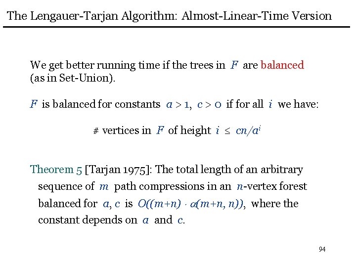
The Lengauer-Tarjan Algorithm: Almost-Linear-Time Version We get better running time if the trees in F are balanced (as in Set-Union). F is balanced for constants a > 1, c > 0 if for all i we have: # vertices in F of height i cn/ai Theorem 5 [Tarjan 1975]: The total length of an arbitrary sequence of m path compressions in an n-vertex forest balanced for a, c is O((m+n) (m+n, n)), where the constant depends on a and c. 94

Linear-Time Algorithms There are linear-time dominators algorithms both for the RAM Model and the Pointer-Machine Model. • Based on LT, but much more complicated. • First published algorithms that claimed linear-time, in fact didn’t achieve that bound. RAM: Harel [1985] Alstrup, Harel, Lauridsen and Thorup [1999] Pointer-Machine: Buchsbaum, Kaplan, Rogers and Westbrook [1998] Georgiadis and Tarjan [2004] 95

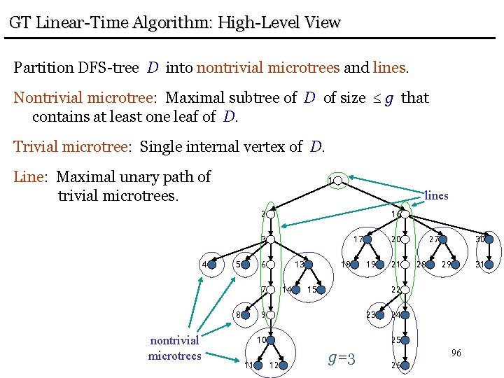
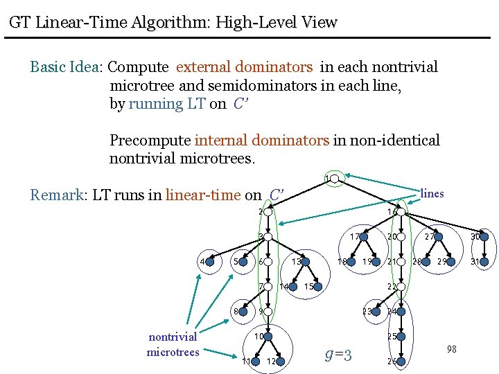
GT Linear-Time Algorithm: High-Level View Partition DFS-tree D into nontrivial microtrees and lines. Nontrivial microtree: Maximal subtree of D of size g that contains at least one leaf of D. Trivial microtree: Single internal vertex of D. Line: Maximal unary path of trivial microtrees. 1 lines 2 16 3 4 5 17 6 13 7 8 nontrivial microtrees 14 18 19 15 21 27 28 30 29 22 9 23 10 11 20 24 25 12 g=3 96 26 31

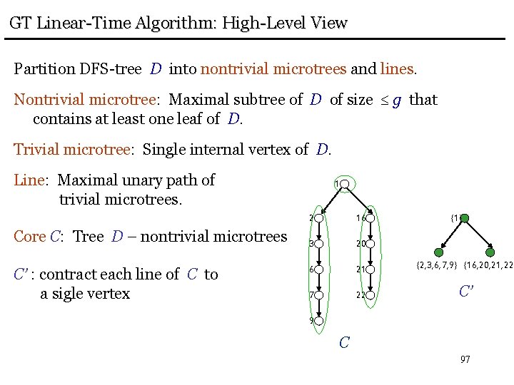
GT Linear-Time Algorithm: High-Level View Partition DFS-tree D into nontrivial microtrees and lines. Nontrivial microtree: Maximal subtree of D of size g that contains at least one leaf of D. Trivial microtree: Single internal vertex of D. Line: Maximal unary path of trivial microtrees. Core C: Tree D – nontrivial microtrees C’ : contract each line of C to a sigle vertex 1 2 16 {1} 3 20 6 21 {2, 3, 6, 7, 9} {16, 20, 21, 22} 7 22 C’ 9 C 97

GT Linear-Time Algorithm: High-Level View Basic Idea: Compute external dominators in each nontrivial microtree and semidominators in each line, by running LT on C’ Precompute internal dominators in non-identical nontrivial microtrees. 1 Remark: LT runs in linear-time on C’ lines 2 16 3 4 5 17 6 13 7 8 nontrivial microtrees 14 18 19 15 21 27 28 30 29 22 9 23 10 11 20 24 25 12 g=3 98 26 31

The Lengauer-Tarjan Algorithm: Almost-Linear-Time Version Back to the O(n (m, n))-time version of LT… We give the details of a data structure that achieves asymptotically faster link() and eval() 99

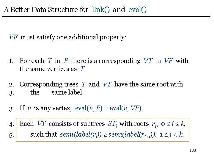
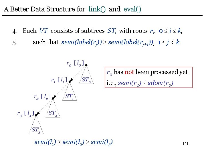
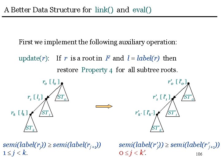
A Better Data Structure for link() and eval() VF must satisfy one additional property: 1. For each T in F there is a corresponding VT in VF with the same vertices as T. 2. Corresponding trees T and VT have the same root with 3. the same label. 3. If v is any vertex, eval(v, F) = eval(v, VF). 4. Each VT consists of subtrees STi with roots ri, 0 i k, 5. such that semi(label(rj)) semi(label(rj+1)), 1 j < k. 100

A Better Data Structure for link() and eval() 4. Each VT consists of subtrees STi with roots ri, 0 i k, 5. such that semi(label(rj)) semi(label(rj+1)), 1 j < k. r 0 has not been processed yet i. e. , semi(r 0) sdom(r 0) semi(l 1) semi(l 2) semi(l 3) 101

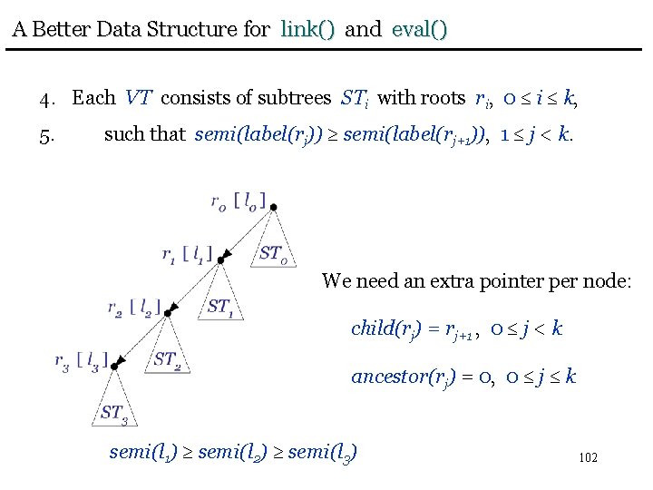
A Better Data Structure for link() and eval() 4. Each VT consists of subtrees STi with roots ri, 0 i k, 5. such that semi(label(rj)) semi(label(rj+1)), 1 j < k. We need an extra pointer per node: child(rj) = rj+1 , 0 j < k ancestor(rj) = 0, 0 j k semi(l 1) semi(l 2) semi(l 3) 102

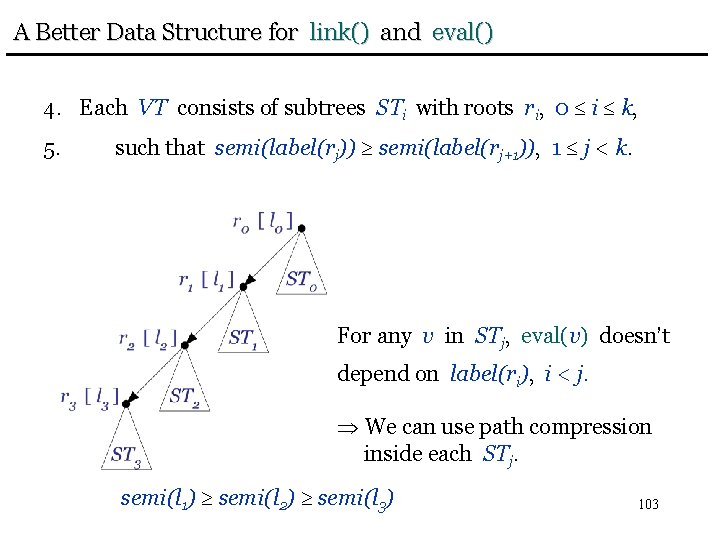
A Better Data Structure for link() and eval() 4. Each VT consists of subtrees STi with roots ri, 0 i k, 5. such that semi(label(rj)) semi(label(rj+1)), 1 j < k. For any v in STj, eval(v) doesn’t depend on label(ri), i < j. We can use path compression inside each STj. semi(l 1) semi(l 2) semi(l 3) 103

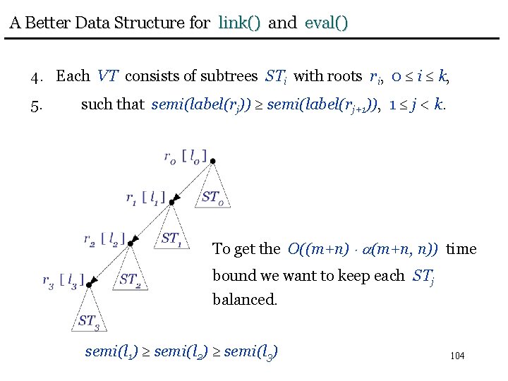
A Better Data Structure for link() and eval() 4. Each VT consists of subtrees STi with roots ri, 0 i k, 5. such that semi(label(rj)) semi(label(rj+1)), 1 j < k. To get the O((m+n) (m+n, n)) time bound we want to keep each STj balanced. semi(l 1) semi(l 2) semi(l 3) 104

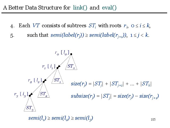
A Better Data Structure for link() and eval() 4. Each VT consists of subtrees STi with roots ri, 0 i k, 5. such that semi(label(rj)) semi(label(rj+1)), 1 j < k. size(rj) = |STj| + |STj+1| + … + |STk| subsize(rj) = |STj| = size(rj) – size(rj+1) semi(l 1) semi(l 2) semi(l 3) 105

A Better Data Structure for link() and eval() First we implement the following auxiliary operation: update(r): If r is a root in F and l = label(r) then restore Property 4 for all subtree roots. semi(label(rj)) semi(label(rj+1)) 1 j < k. semi(label(r’j)) semi(label(r’j+1)) 0 j < k’. 106

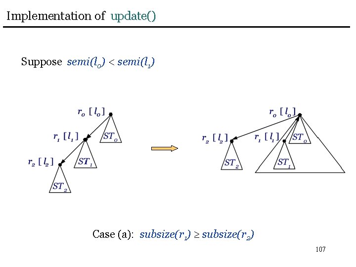
Implementation of update() Suppose semi(l 0) < semi(l 1) Case (a): subsize(r 1) subsize(r 2) 107

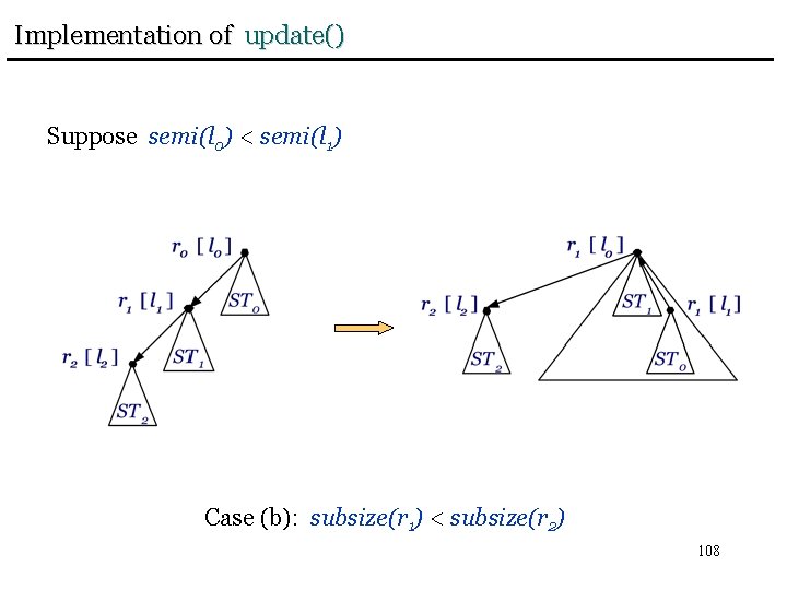
Implementation of update() Suppose semi(l 0) < semi(l 1) Case (b): subsize(r 1) < subsize(r 2) 108

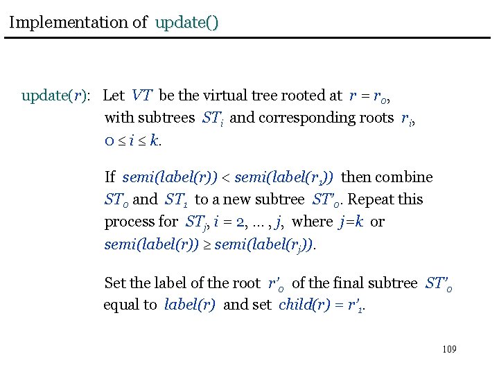
Implementation of update() update(r): Let VT be the virtual tree rooted at r = r 0, with subtrees STi and corresponding roots ri, 0 i k. If semi(label(r)) < semi(label(r 1)) then combine ST 0 and ST 1 to a new subtree ST’ 0. Repeat this process for STj, i = 2, … , j, where j=k or semi(label(r)) semi(label(rj)). Set the label of the root r’ 0 of the final subtree ST’ 0 equal to label(r) and set child(r) = r’ 1. 109

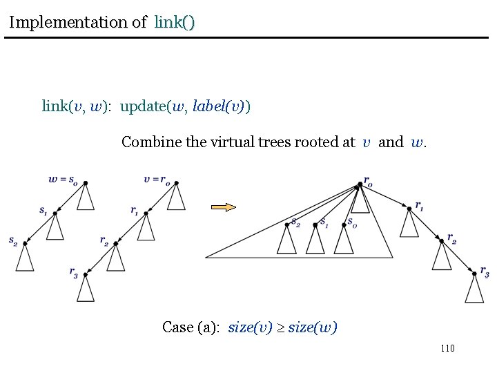
Implementation of link() link(v, w): update(w, label(v)) Combine the virtual trees rooted at v and w. Case (a): size(v) size(w) 110

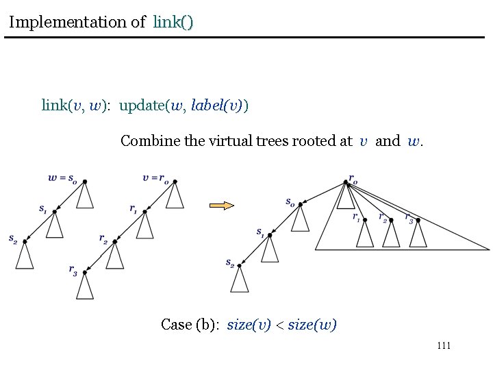
Implementation of link() link(v, w): update(w, label(v)) Combine the virtual trees rooted at v and w. Case (b): size(v) < size(w) 111

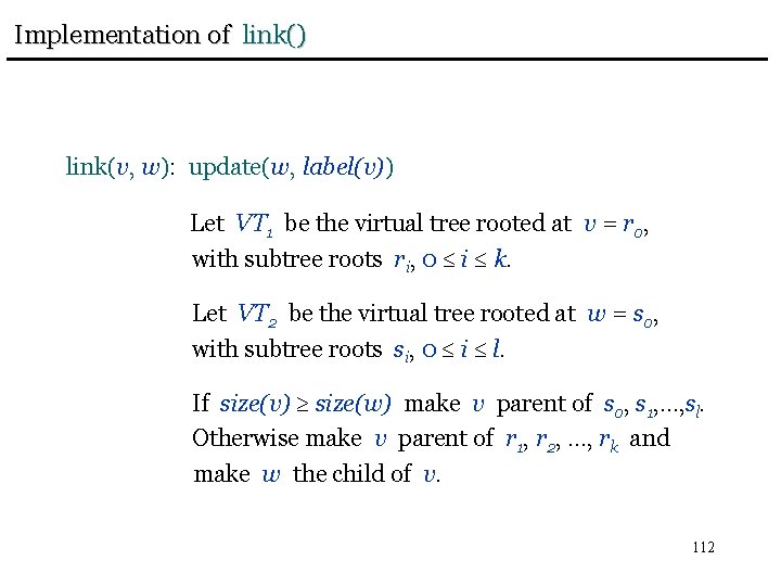
Implementation of link() link(v, w): update(w, label(v)) Let VT 1 be the virtual tree rooted at v = r 0, with subtree roots ri, 0 i k. Let VT 2 be the virtual tree rooted at w = s 0, with subtree roots si, 0 i l. If size(v) size(w) make v parent of s 0, s 1, …, sl. Otherwise make v parent of r 1, r 2, …, rk and make w the child of v. 112

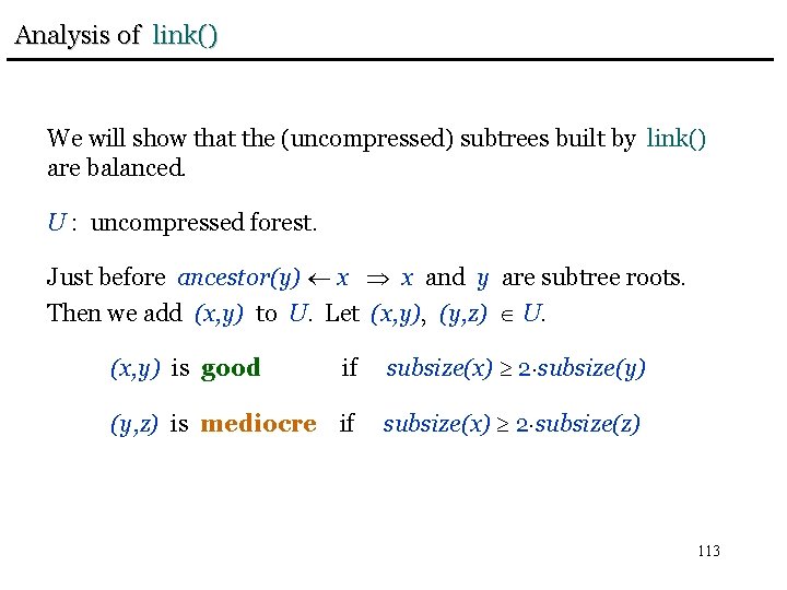
Analysis of link() We will show that the (uncompressed) subtrees built by link() are balanced. U : uncompressed forest. Just before ancestor(y) x x and y are subtree roots. Then we add (x, y) to U. Let (x, y), (y, z) U. if subsize(x) 2 subsize(y) (y, z) is mediocre if subsize(x) 2 subsize(z) (x, y) is good 113

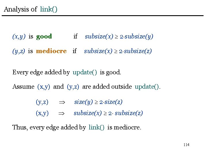
Analysis of link() if subsize(x) 2 subsize(y) (y, z) is mediocre if subsize(x) 2 subsize(z) (x, y) is good Every edge added by update() is good. Assume (x, y) and (y, z) are added outside update(). (y, z) size(y) 2 size(z) (x, y) subsize(x) 2 subsize(z) Thus, every edge added by link() is mediocre. 114

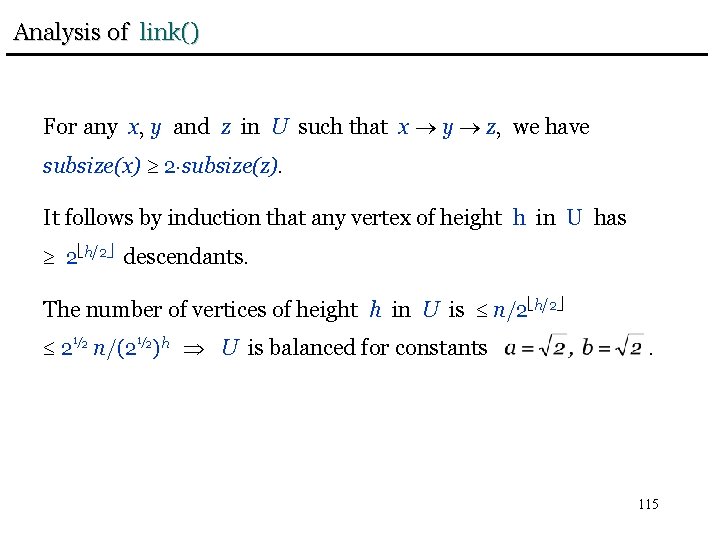
Analysis of link() For any x, y and z in U such that x y z, we have subsize(x) 2 subsize(z). It follows by induction that any vertex of height h in U has 2 h/2 descendants. The number of vertices of height h in U is n/2 h/2 2½ n/(2½)h U is balanced for constants . 115

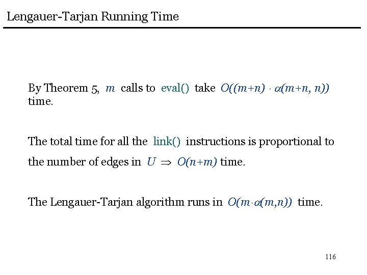
Lengauer-Tarjan Running Time By Theorem 5, m calls to eval() take O((m+n) (m+n, n)) time. The total time for all the link() instructions is proportional to the number of edges in U O(n+m) time. The Lengauer-Tarjan algorithm runs in O(m (m, n)) time. 116