Finding A Chessboard An Introduction To Computer Vision

Finding A Chessboard: An Introduction To Computer Vision Martin C. Martin March 9, 2005

Motivation & Inspiration • A spare time project, because I thought it would be fun • Project: Chess against the computer, where board and your pieces are real, it’s pieces are projected • Working so far: very robust localizing of chessboard (full 3 D location and orientation) March 9, 2005 6

Requirements • Interaction should be as natural as possible – E. g. pieces don’t have to be centered in their squares, or even completely in them • Should be easy to set up and give demonstrations – Little calibration as possible – Work in many lighting conditions – Although only with this board and pieces • Camera needs to be at angle to board • Board made by my father just before he met my mother – My brother and I learned to play on it • I’m not a big chess fan, I just like project March 9, 2005 7

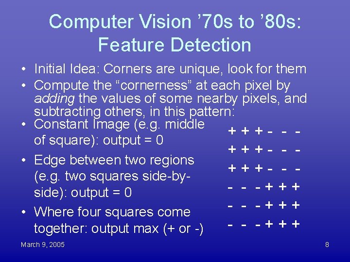
Computer Vision ’ 70 s to ’ 80 s: Feature Detection • Initial Idea: Corners are unique, look for them • Compute the “cornerness” at each pixel by adding the values of some nearby pixels, and subtracting others, in this pattern: • Constant Image (e. g. middle +++- - of square): output = 0 +++- - • Edge between two regions + + + (e. g. two squares side-by- - -+++ side): output = 0 - - -+++ • Where four squares come - - -+++ together: output max (+ or -) March 9, 2005 8

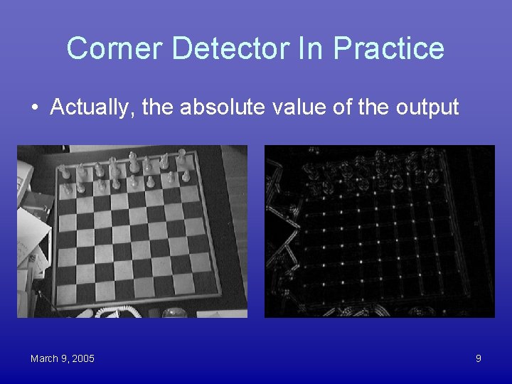
Corner Detector In Practice • Actually, the absolute value of the output March 9, 2005 9

Problems With Corner Detection • • Edge effects Strong response for some non-corners Easily obscured by pieces, hand How to link them up when many are obscured? • Go back to something older: Find edges March 9, 2005 10

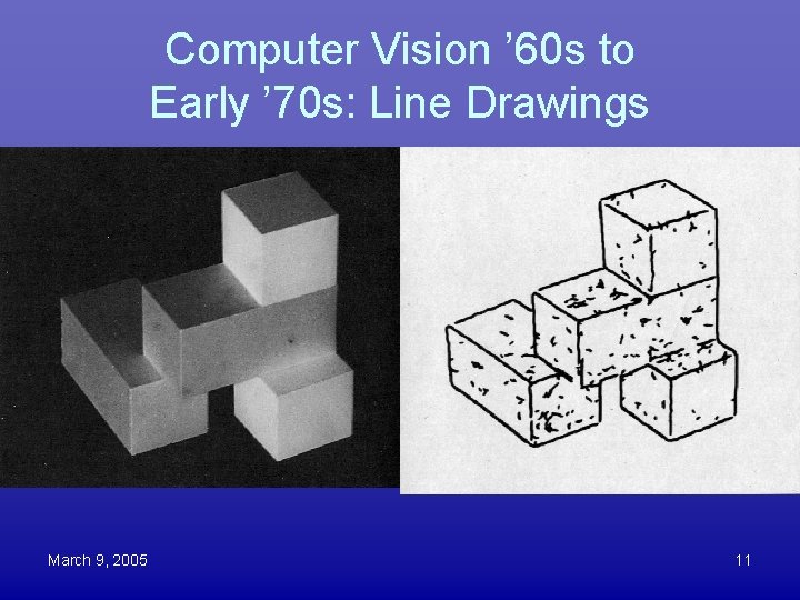
Computer Vision ’ 60 s to Early ’ 70 s: Line Drawings March 9, 2005 11

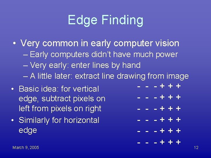
Edge Finding • Very common in early computer vision – Early computers didn’t have much power – Very early: enter lines by hand – A little later: extract line drawing from image • Basic idea: for vertical edge, subtract pixels on left from pixels on right • Similarly for horizontal edge March 9, 2005 - - -+++ -+++ 12

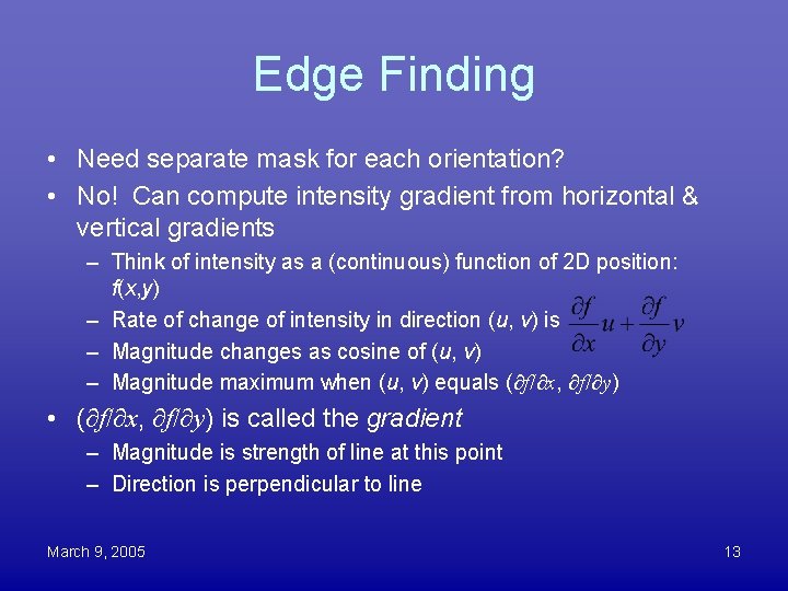
Edge Finding • Need separate mask for each orientation? • No! Can compute intensity gradient from horizontal & vertical gradients – Think of intensity as a (continuous) function of 2 D position: f(x, y) – Rate of change of intensity in direction (u, v) is – Magnitude changes as cosine of (u, v) – Magnitude maximum when (u, v) equals (∂f/∂x, ∂f/∂y) • (∂f/∂x, ∂f/∂y) is called the gradient – Magnitude is strength of line at this point – Direction is perpendicular to line March 9, 2005 13

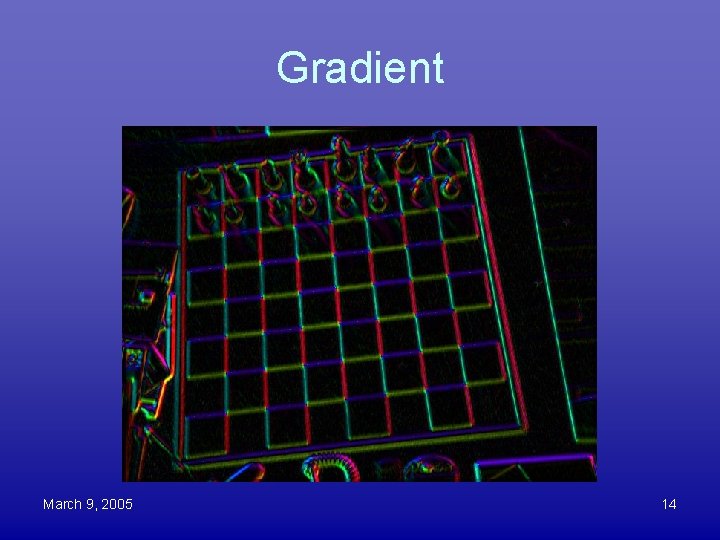
Gradient March 9, 2005 14

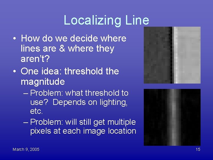
Localizing Line • How do we decide where lines are & where they aren’t? • One idea: threshold the magnitude – Problem: what threshold to use? Depends on lighting, etc. – Problem: will still get multiple pixels at each image location March 9, 2005 15

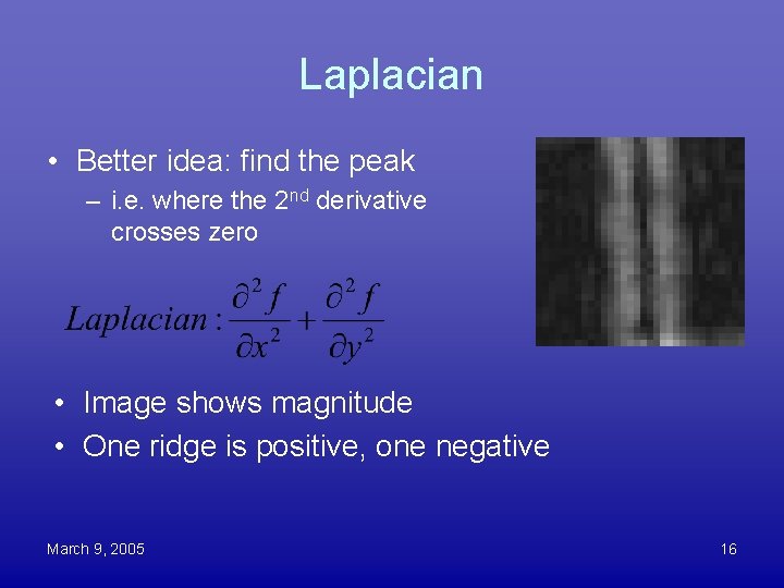
Laplacian • Better idea: find the peak – i. e. where the 2 nd derivative crosses zero • Image shows magnitude • One ridge is positive, one negative March 9, 2005 16

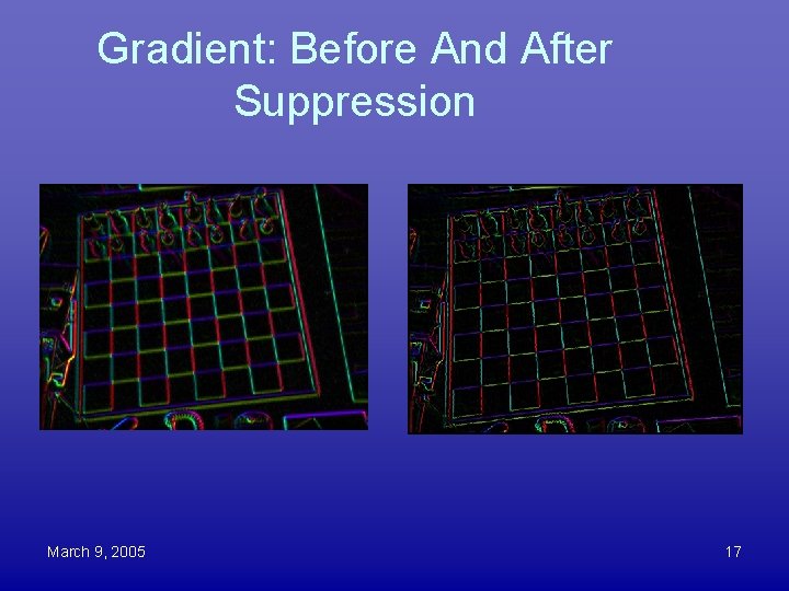
Gradient: Before And After Suppression March 9, 2005 17

Extracting Whole Lines • So Far: intensity image “lineness” image • Next: “lineness” image list of lines • Need to accumulate contributions from across image – Could be many gaps • Want to extract position & orientation of lines – Boundaries won’t be robust, so consider lines to run across the entire image March 9, 2005 18

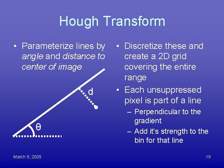
Hough Transform • Parameterize lines by angle and distance to center of image d θ March 9, 2005 • Discretize these and create a 2 D grid covering the entire range • Each unsuppressed pixel is part of a line – Perpendicular to the gradient – Add it’s strength to the bin for that line 19

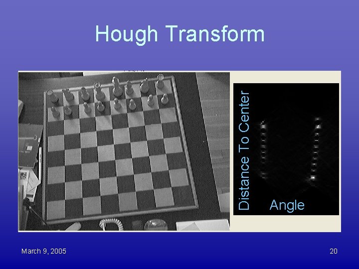
Distance To Center Hough Transform March 9, 2005 Angle 20

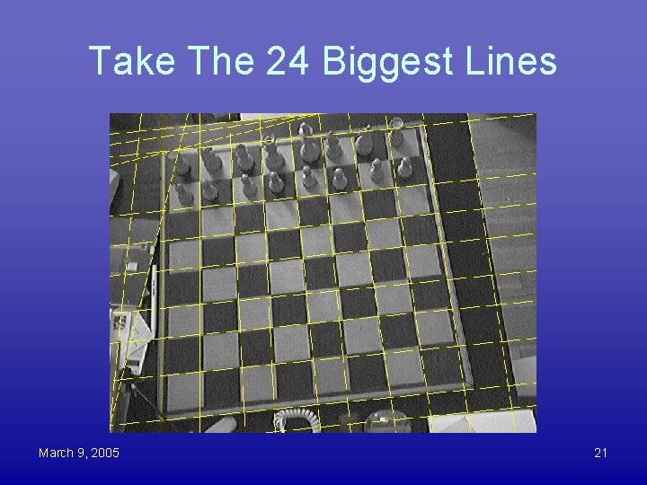
Take The 24 Biggest Lines March 9, 2005 21

Demonstration March 9, 2005 22

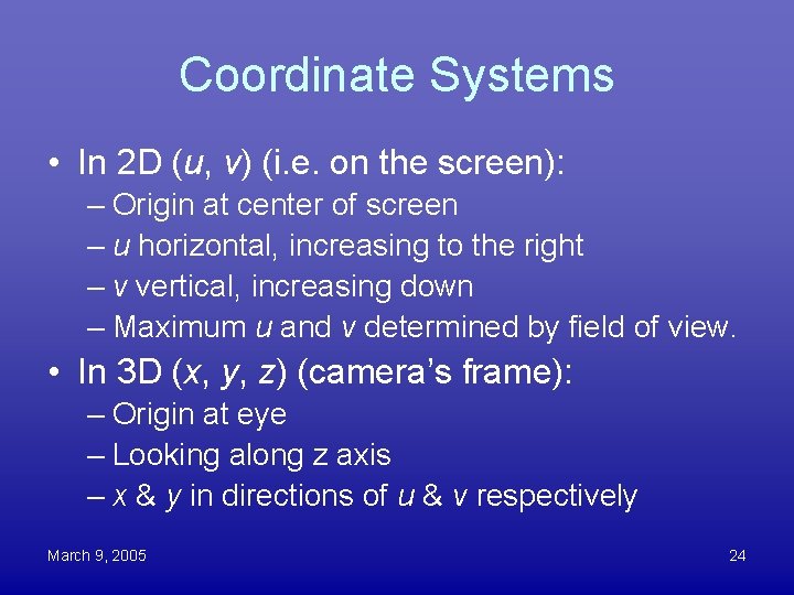
Coordinate Systems • In 2 D (u, v) (i. e. on the screen): – Origin at center of screen – u horizontal, increasing to the right – v vertical, increasing down – Maximum u and v determined by field of view. • In 3 D (x, y, z) (camera’s frame): – Origin at eye – Looking along z axis – x & y in directions of u & v respectively March 9, 2005 24

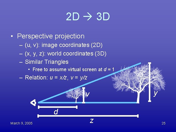
2 D 3 D • Perspective projection – (u, v): image coordinates (2 D) – (x, y, z): world coordinates (3 D) – Similar Triangles • Free to assume virtual screen at d = 1 – Relation: u = x/z, v = y/z y v d March 9, 2005 z 25

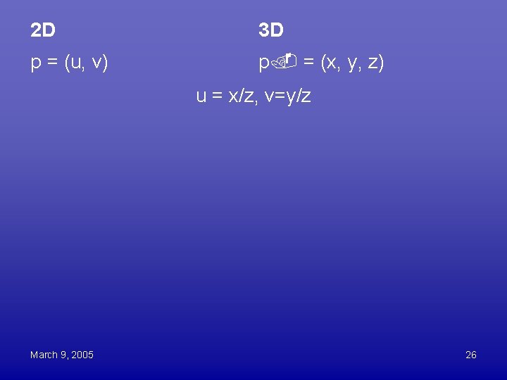
2 D 3 D p = (u, v) p = (x, y, z) u = x/z, v=y/z March 9, 2005 26

Lines in 3 D map to lines on screen • Proof: the 3 D line, plus the origin (eye), form a plane. • All light rays from the 3 D line to the eye are in this plane. • The intersection of that plane and the image plane form a line March 9, 2005 27

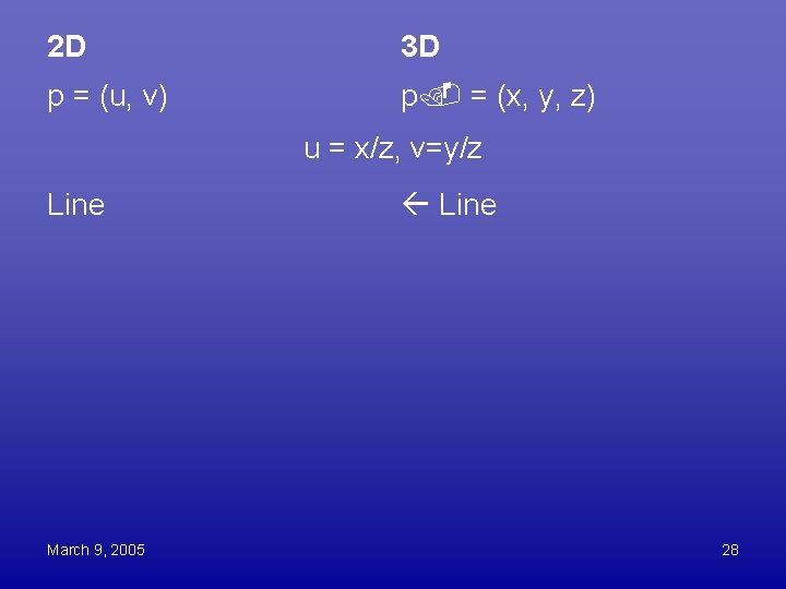
2 D 3 D p = (u, v) p = (x, y, z) u = x/z, v=y/z Line March 9, 2005 Line 28

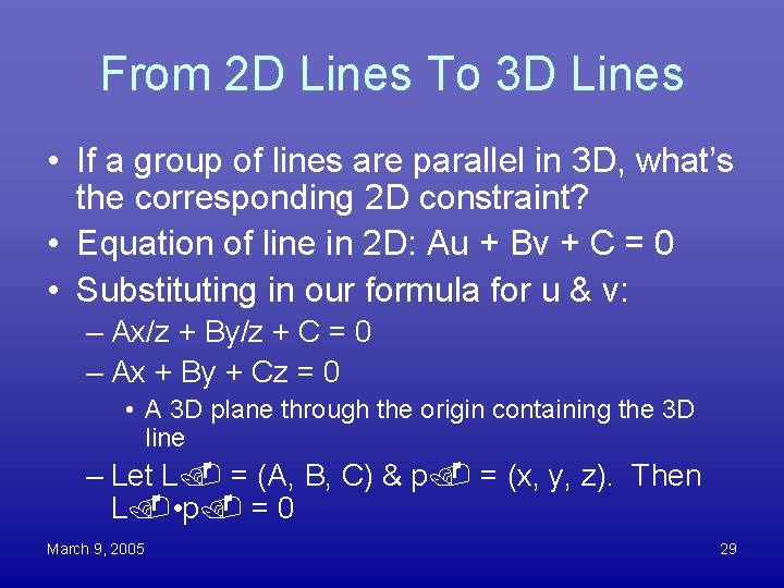
From 2 D Lines To 3 D Lines • If a group of lines are parallel in 3 D, what’s the corresponding 2 D constraint? • Equation of line in 2 D: Au + Bv + C = 0 • Substituting in our formula for u & v: – Ax/z + By/z + C = 0 – Ax + By + Cz = 0 • A 3 D plane through the origin containing the 3 D line – Let L = (A, B, C) & p = (x, y, z). Then L • p = 0 March 9, 2005 29

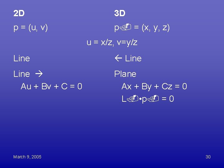
2 D 3 D p = (u, v) p = (x, y, z) u = x/z, v=y/z Line Au + Bv + C = 0 Plane Ax + By + Cz = 0 L • p = 0 March 9, 2005 30

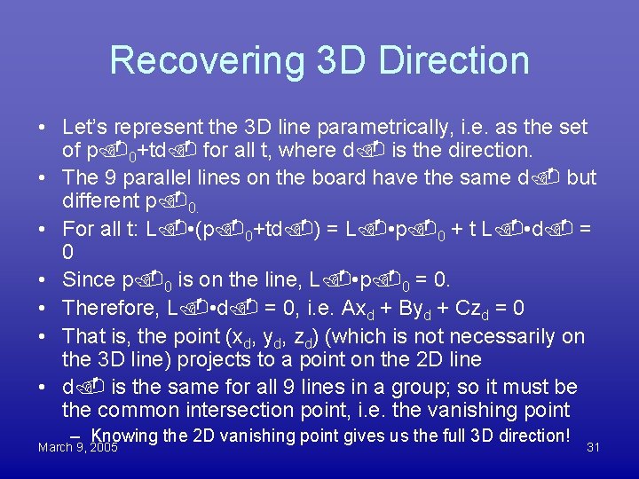
Recovering 3 D Direction • Let’s represent the 3 D line parametrically, i. e. as the set of p 0+td for all t, where d is the direction. • The 9 parallel lines on the board have the same d but different p 0. • For all t: L • (p 0+td ) = L • p 0 + t L • d = 0 • Since p 0 is on the line, L • p 0 = 0. • Therefore, L • d = 0, i. e. Axd + Byd + Czd = 0 • That is, the point (xd, yd, zd) (which is not necessarily on the 3 D line) projects to a point on the 2 D line • d is the same for all 9 lines in a group; so it must be the common intersection point, i. e. the vanishing point – Knowing the 2 D vanishing point gives us the full 3 D direction! March 9, 2005 31

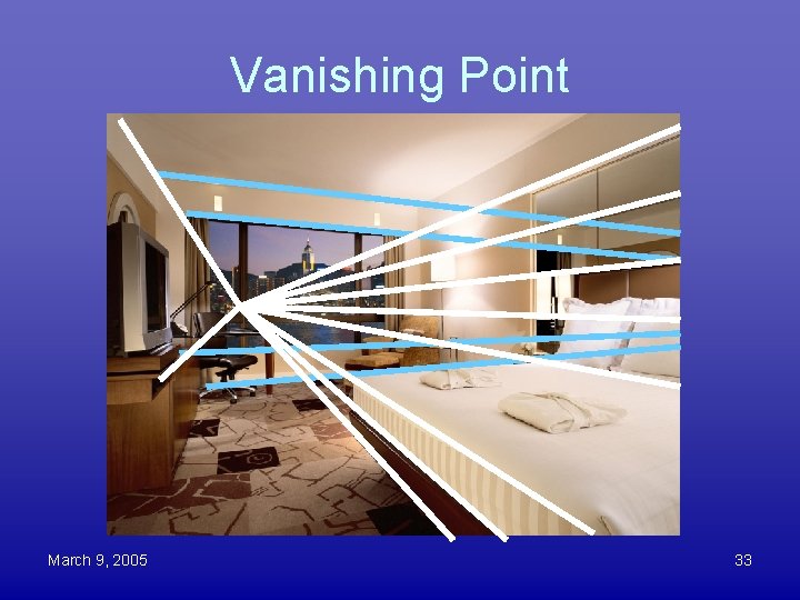
Vanishing Point March 9, 2005 33

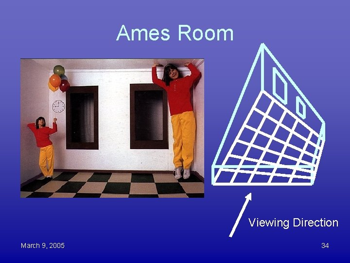
Ames Room Viewing Direction March 9, 2005 34

2 D 3 D p = (u, v) p = (x, y, z) u = x/z, v=y/z Line Au + Bv + C = 0 Plane Ax + By + Cz = 0 L • p = 0 Parallel Lines Common Direction Common Intersection Vanishing Point March 9, 2005 35

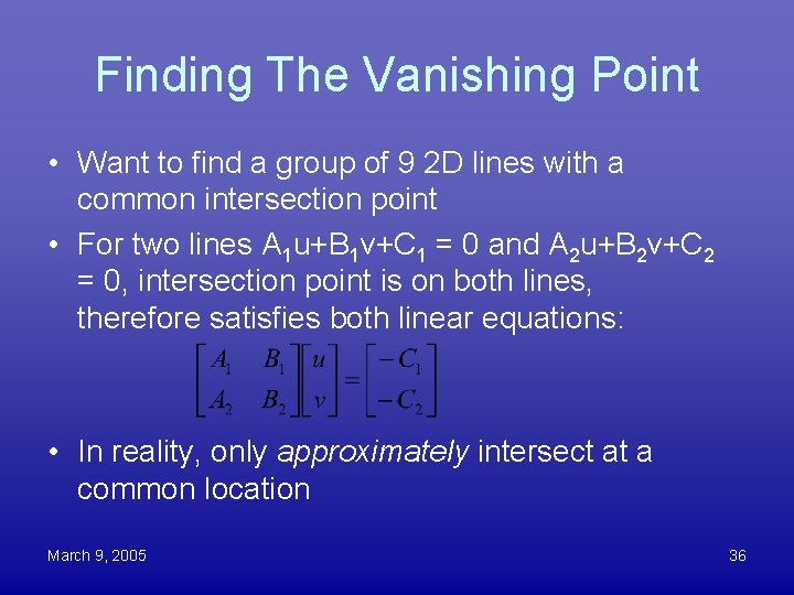
Finding The Vanishing Point • Want to find a group of 9 2 D lines with a common intersection point • For two lines A 1 u+B 1 v+C 1 = 0 and A 2 u+B 2 v+C 2 = 0, intersection point is on both lines, therefore satisfies both linear equations: • In reality, only approximately intersect at a common location March 9, 2005 36

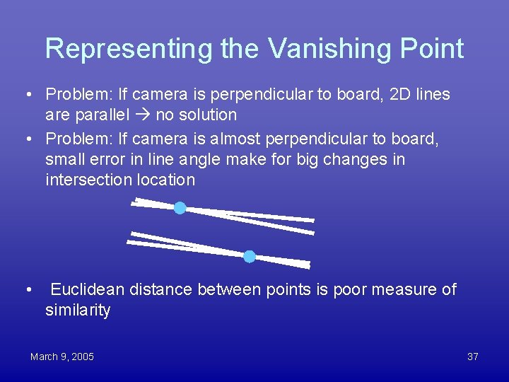
Representing the Vanishing Point • Problem: If camera is perpendicular to board, 2 D lines are parallel no solution • Problem: If camera is almost perpendicular to board, small error in line angle make for big changes in intersection location • Euclidean distance between points is poor measure of similarity March 9, 2005 37

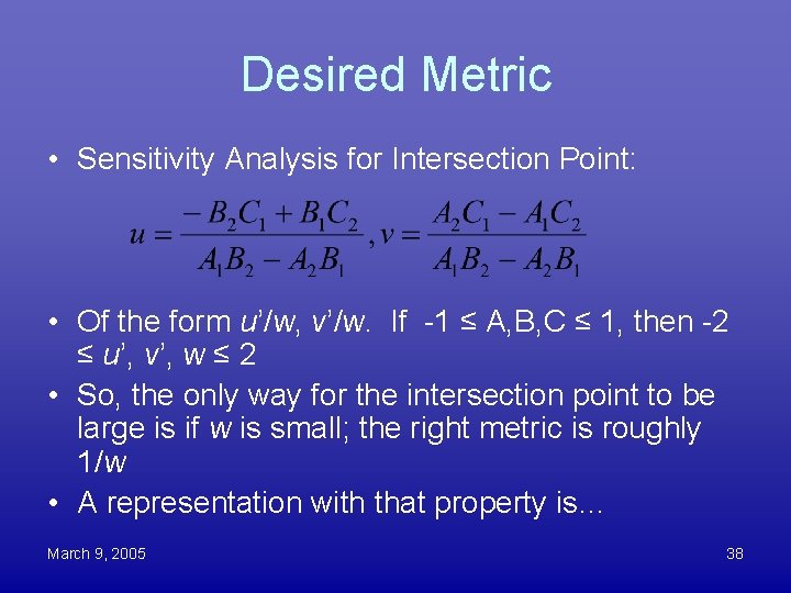
Desired Metric • Sensitivity Analysis for Intersection Point: • Of the form u’/w, v’/w. If -1 ≤ A, B, C ≤ 1, then -2 ≤ u’, v’, w ≤ 2 • So, the only way for the intersection point to be large is if w is small; the right metric is roughly 1/w • A representation with that property is… March 9, 2005 38

Homogeneous Coordinates • • • Introduced by August Ferdinand Möbius An example of projective geometry Represent a 2 D point using 3 numbers The point (u, v, w) corresponds to u/w, v/w Formula for perspective projection means any 3 D point is already the homogeneous coordinate of its 2 D projection • Multiplying by a scalar doesn’t change the point: – (cu, cv, cw) represents same 2 D point as (u, v, w) March 9, 2005 39

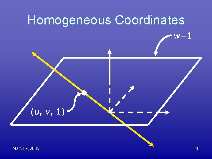
Homogeneous Coordinates w=1 (u, v, 1) March 9, 2005 40

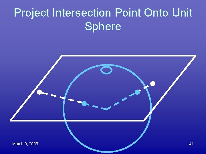
Project Intersection Point Onto Unit Sphere March 9, 2005 41

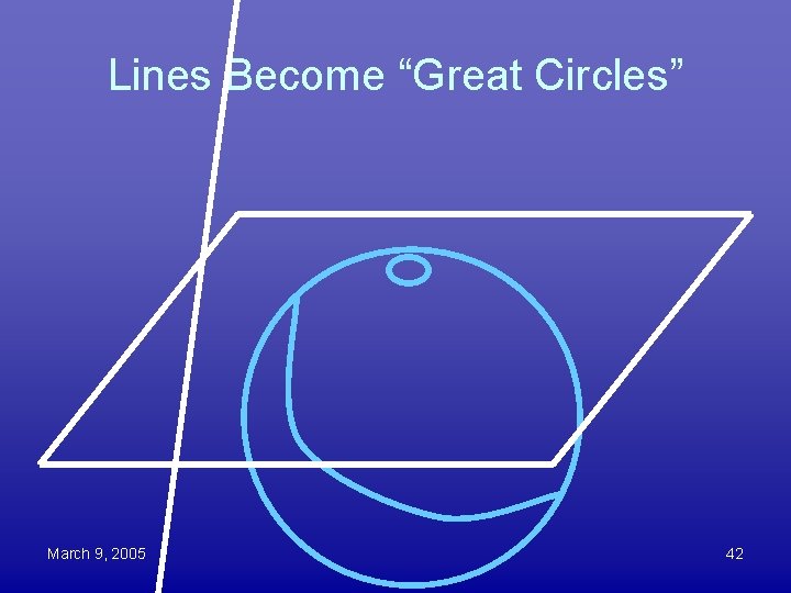
Lines Become “Great Circles” March 9, 2005 42

Clustering: Computer Vision In The Nineties • 60 s and 70 s: Promise of human equivalence right around the corner • 80 s: Backlash against AI – Like an “internet startup” now • 90 s: Extensions of existing engineering techniques – Applied statistics: Bayesian Networks – Control Theory: Reinforcement Learning March 9, 2005 43

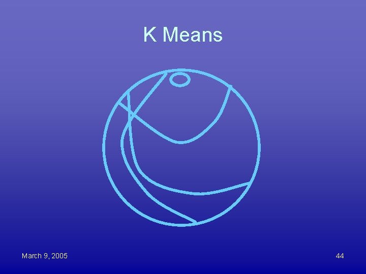
K Means March 9, 2005 44

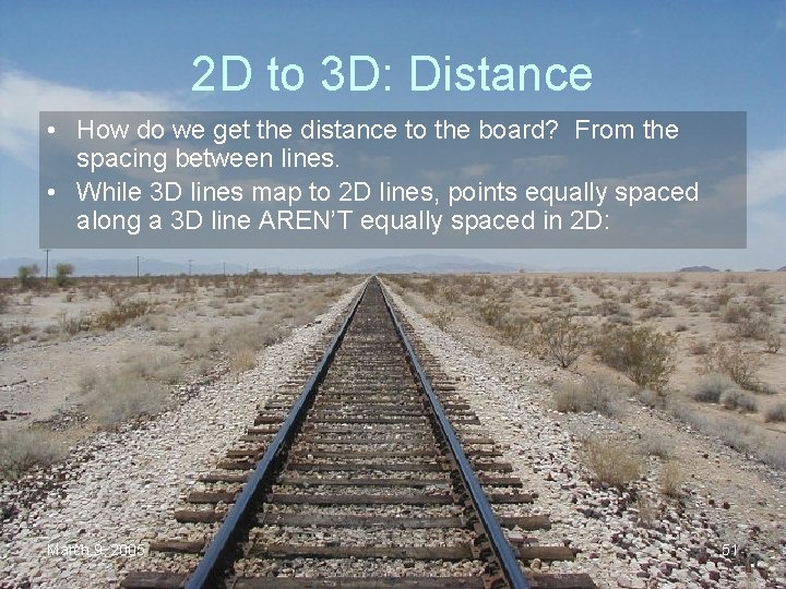
2 D to 3 D: Distance • How do we get the distance to the board? From the spacing between lines. • While 3 D lines map to 2 D lines, points equally spaced along a 3 D line AREN’T equally spaced in 2 D: March 9, 2005 51

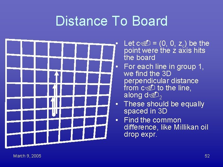
Distance To Board • Let c = (0, 0, zc) be the point were the z axis hits the board • For each line in group 1, we find the 3 D perpendicular distance from c to the line, along d 2 • These should be equally spaced in 3 D • Find the common difference, like Millikan oil drop expr. March 9, 2005 52

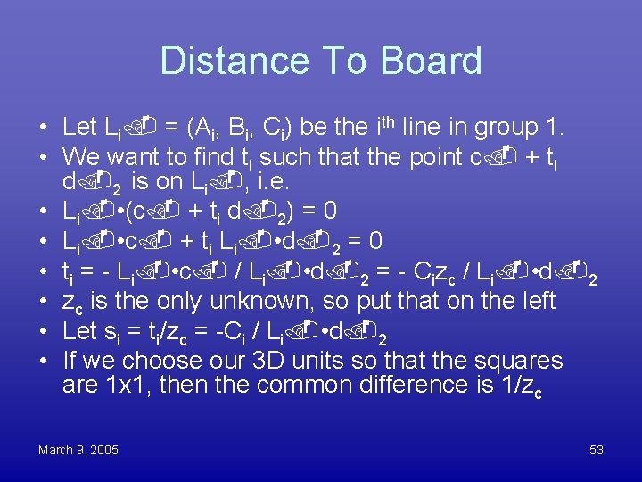
Distance To Board • Let Li = (Ai, Bi, Ci) be the ith line in group 1. • We want to find ti such that the point c + ti d 2 is on Li , i. e. • Li • (c + ti d 2) = 0 • Li • c + ti Li • d 2 = 0 • ti = - Li • c / Li • d 2 = - Cizc / Li • d 2 • zc is the only unknown, so put that on the left • Let si = ti/zc = -Ci / Li • d 2 • If we choose our 3 D units so that the squares are 1 x 1, then the common difference is 1/zc March 9, 2005 53

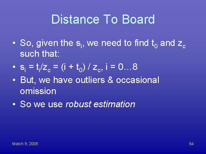
Distance To Board • So, given the si, we need to find t 0 and zc such that: • si = ti/zc = (i + t 0) / zc, i = 0… 8 • But, we have outliers & occasional omission • So we use robust estimation March 9, 2005 54

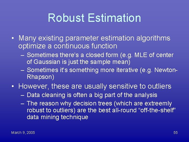
Robust Estimation • Many existing parameter estimation algorithms optimize a continuous function – Sometimes there’s a closed form (e. g. MLE of center of Gaussian is just the sample mean) – Sometimes it’s something more iterative (e. g. Newton. Rhapson) • However, these are usually sensitive to outliers – Data cleaning is often a big part of the analysis – The reason why decision trees (which are extreemly robust to outliers) are the best all-round “off-the-shelf” data mining technique March 9, 2005 55

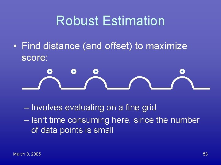
Robust Estimation • Find distance (and offset) to maximize score: – Involves evaluating on a fine grid – Isn’t time consuming here, since the number of data points is small March 9, 2005 56